Evolutionary trade-offs in dormancy phenology
- UMR 7178, Centre National de la Recherche Scientifique, Institut Pluridisciplinaire Hubert CURIEN, Université de Strasbourg, France
- Department of Biological Sciences, Auburn University, United States
- Department of Interdisciplinary Life Sciences, Research Institute of Wildlife Ecology, University of Veterinary Medicine Vienna, Austria
- Energetic Lab, Department of Biology, Northern Michigan University, United States
Figures
Figure 1
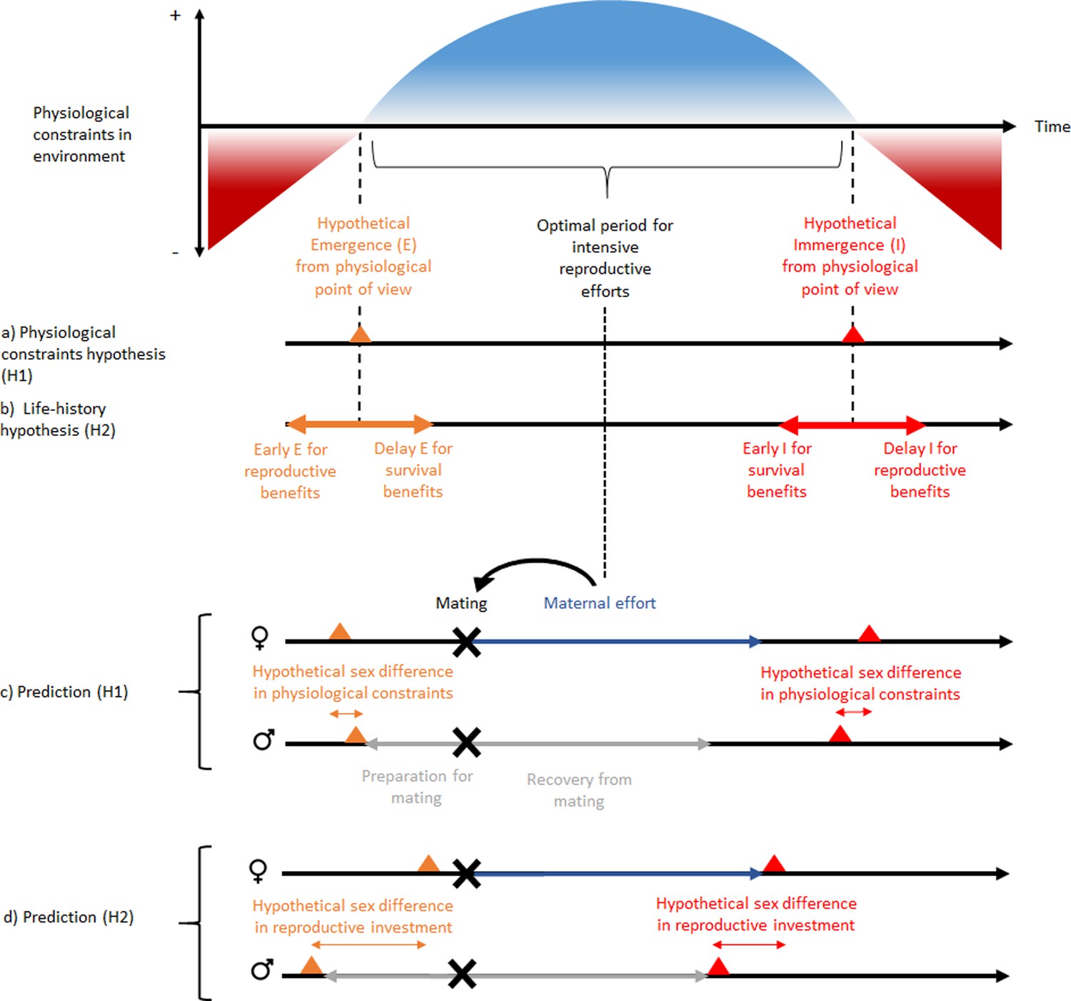
Schematic representation of ‘the physiological constraint hypothesis’ and ‘the lifehistory hypothesis’ and their predictions.
Physiological constraints in the environment refers to variation over time of the energetic balance (mainly for heterothermic endotherms) and the thermal window favorable to activity (mainly for ectotherms). Hypothesis H1 assumes that dormancy phenology occurs at the time of transition between favorable and unfavorable energetic or thermal conditions or vice versa. It predicts that the sex difference in dormancy phenology is explained by sex differences in physiological constraints, and that reproductive investment should be independent of this sex difference in phenology. In contrast, hypothesis H2 predicts that a phenology that would occur before or after the energetic transition may be associated with benefits to survival or reproduction. It predicts that the sex difference in dormancy phenology is associated with a sex difference in reproductive investment. This pattern is expected for species without paternal effort. But the concept can be applied to other types of mating strategies. The hibernation phenology presented for prediction (H1) are those expected for hibernating mammals. Note that the magnitude and order of sex differences in phenology is not an expected general trend, because it is assumed to vary between species according to beneficial envioronmental conditions for energy demand (prediction H1) and reproductive investment (prediction H2). Nevertheless, the sex difference is assumed to be smaller with the H1 prediction because there is less sex difference in energy demand than in reproductive investment. Black, gray, and dark blue horizontal arrows represent respectively time over the year, reproductive investment in males and reproductive investment in females. Black, gray, and dark blue horizontal arrows represent respectively time over the year, reproductive investment in males and reproductive investment in females. Red and orange triangles represent respectively immergence and emergence timing and black cross represent mating timing.
Figure 2
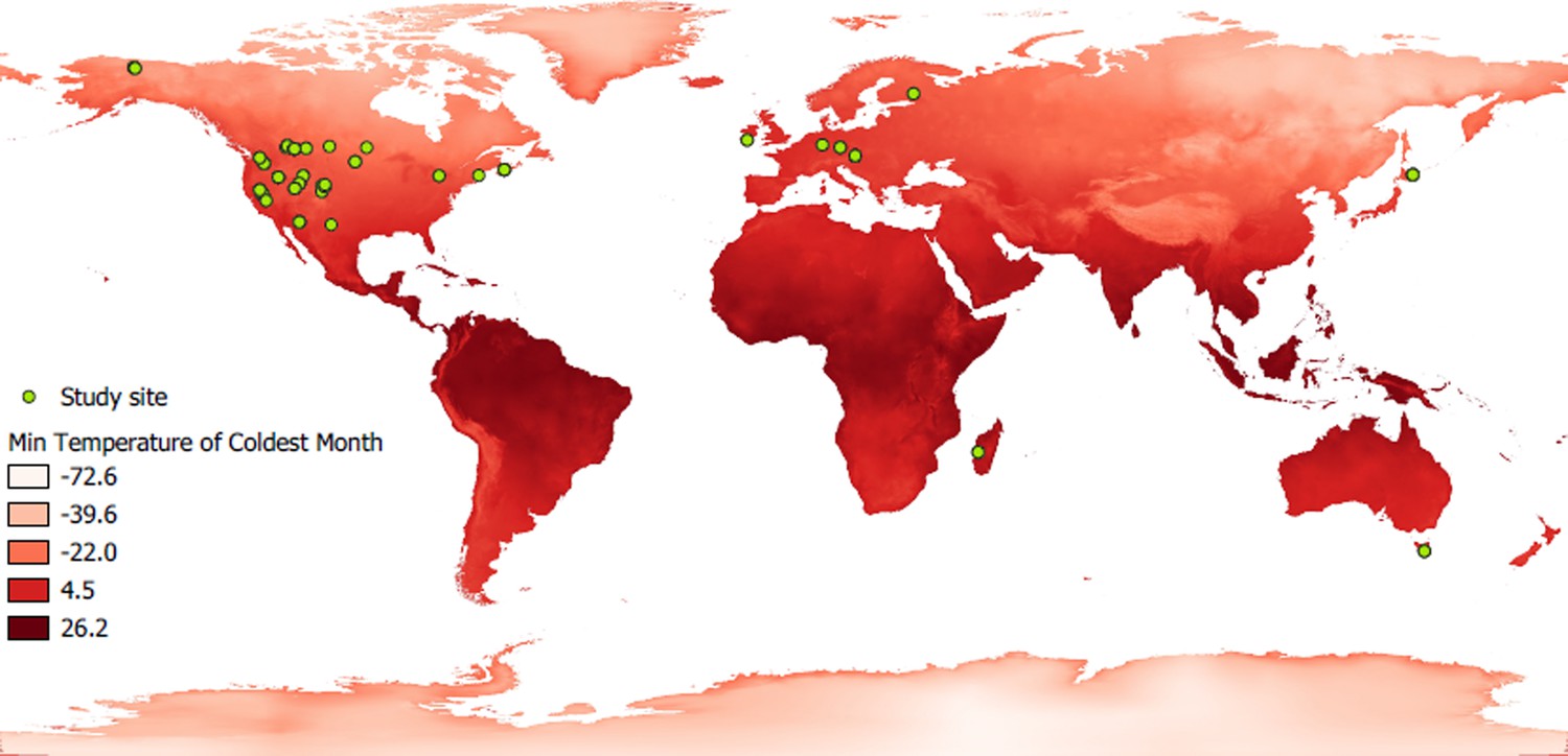
World map showing the study sites of the hibernating species studied.
Green dots cindicate the location of study sites. A red gradient represents the variation in minimum ambient temperature, a parameter used in this study.
Figure 3
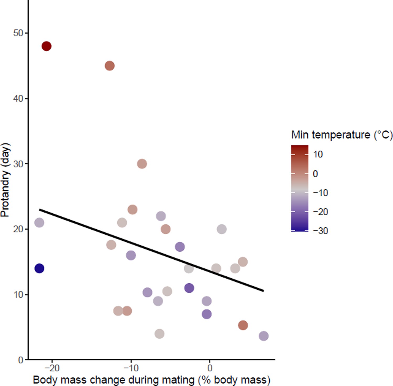
Effects of body mass variation during mating on protandry.
The minimum temperatures of the study sites are indicated by a color gradient with the warmest temperatures in red. The regression line in black indicates the effect of body mass variation during mating on protandry. Body mass variation during mating was represented as a percentage of body mass before mating.
-
Figure 3—source data 1
Hibernation phenology, reproduction, body mass and climate data used in Model 1.
- https://cdn.elifesciences.org/articles/89644/elife-89644-fig3-data1-v1.docx
Figure 4
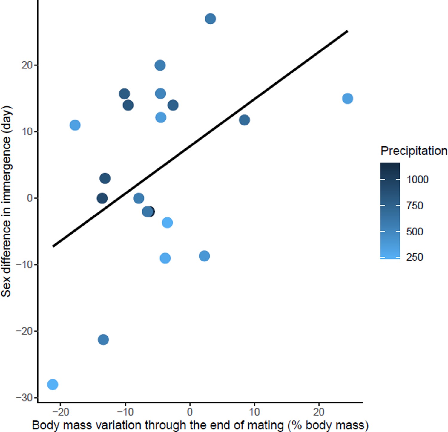
Effects of body mass variation through the end of mating on sex differences in immergence.
Annual precipitation at the study sites are indicated by a color gradient with the highest precipitation in dark blue. The regression line in black indicates the effect of body mass variation through the end of mating on sex difference in immergence. Body mass variation through the end of mating was represented as a percentage of body mass at emergence. Males immerged earlier in species living in an environment with high precipitation (dark blue dots).
-
Figure 4—source data 1
Hibernation phenology, reproduction, body mass and climate data used in Model 2.
- https://cdn.elifesciences.org/articles/89644/elife-89644-fig4-data1-v1.docx
Figure 5
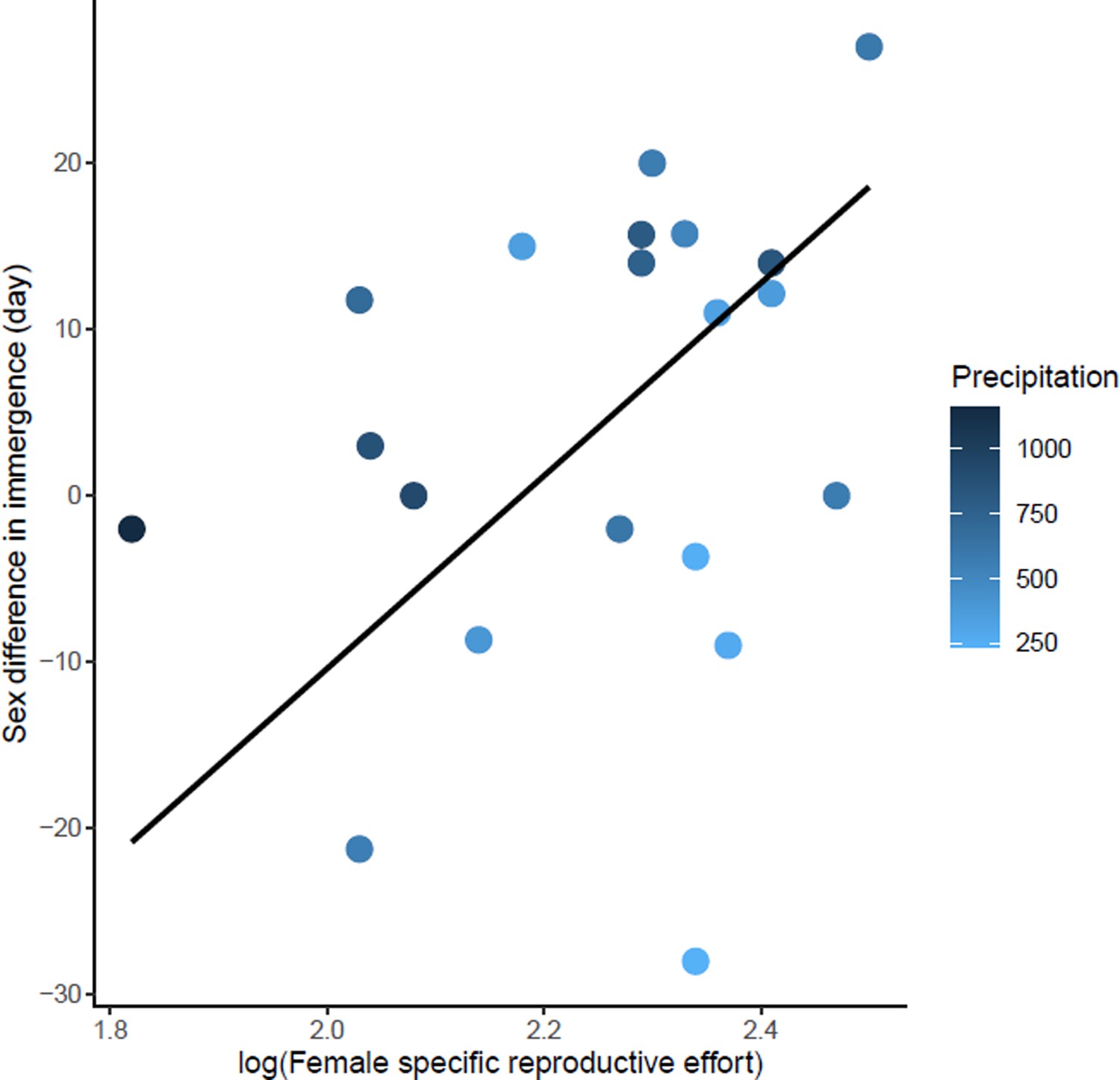
Effects of female specific reproductive effort on sex difference in immergence.
The annual precipitation of the study sites are indicated by a color gradient with the highest precipitation in dark blue. The regression line in black indicates the effect of female specific reproductive effort on sex difference in immergence. Males immerged earlier in species living in an environment with high precipitation (dark blue dots).
-
Figure 5—source data 1
Hibernation phenology, reproduction, body mass and climate data used in Model 3.
- https://cdn.elifesciences.org/articles/89644/elife-89644-fig5-data1-v1.docx
Figure 6
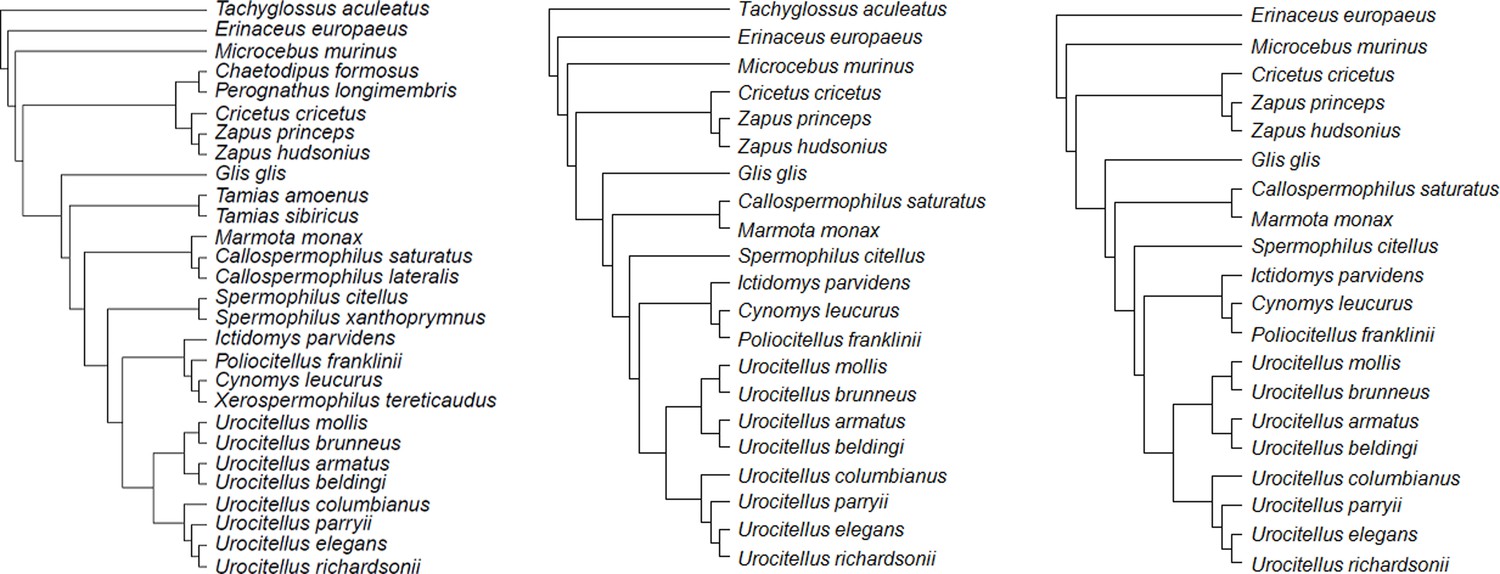
Consensus phylogenetic trees for the species under study: (a) model 1 (b) model 2, and (c) model 3.
Each consensus tree was built from 100 trees obtained from http://vertlife.org/phylosubsets/. Branch lengths were calculated using Grafen’s computations with the ‘ape’ package in R (see Materials and methods).
Tables
Table 1
Regression results for the best models explaining variation in protandry and sex difference in immergence.
The Z standardized model estimates and the phylogenetic effect are reciprocally estimated by β and γM. The abbreviations ‘diff’ and ‘rel’ ‘Min’ stand respectively for ‘difference,’ ‘relative,’ and ‘Minimum.’ A negative value for the sex difference in immergence indicates that males immerge before females and a positive value indicates that females immerge before males. Relative testes mass, Δ body mass before mating, Δ body mass during mating, Δ body mass through the end of mating was represented respectively as a percentage of body mass, body mass at emergence, body mass before mating, and body mass at emergence.
| γ ML | |||||||
|---|---|---|---|---|---|---|---|
| R2 | γ ML | Dependent variable | Independent variable | β±SE | t-value | p-value | |
| Model 1 (28 species) | 0.59 | 0.00 (NA, 0.69) | Protandry | Intercept | 16.31±1.27 | 12.76 | <0.001*** |
| z- Male body mass at emergence | 3.25±1.37 | 2.37 | 0.02* | ||||
| z-D body mass during mating | –3.32±1.39 | –2.38 | 0.02* | ||||
| z-Min temperature | 5.94±1.36 | 4.34 | <0.001*** | ||||
| z- late mating | –2.58±1.41 | –1.83 | 0.08. | ||||
| Model 2 (21 species) | 0.50 | 0.00 (NA, 0.38) | Sex diff in immergence | Intercept | 5.18±2.18 | 2.36 | 0.03* |
| z- log specific reproductive effort | 13.77±3.88 | 3.54 | 0.002** | ||||
| z-D body mass through the end of mating | 9.07±2.37 | 3.81 | 0.001** | ||||
| z- precipitation | 7.67±2.59 | 2.95 | 0.009** | ||||
| z- Maternal effort duration | 12.66±3.58 | 3.52 | 0.002** | ||||
| Model 3 (20 species) | 0.63 | 0.00 (NA, 0.73) | Sex diff in immergence | Intercept | 4.24±1.89 | 2.23 | 0.04* |
| z- log specific reproductive effort | 10.20±2.34 | 4.35 | <0.001*** | ||||
| z-D body mass through the end of mating | 7.05±2.05 | 3.42 | 0.003** | ||||
| z- precipitation | 12.48±2.70 | 4.61 | <0.001*** | ||||
| z-dimorphism at immergence | 4.75±2.42 | 1.96 | 0.06. | ||||
Table 2
Species with dimorphisms biased in favor of males or females and their body mass gain during the year.
Body size dimorphism is calculated as male body size divided by female body size. See section “Sex differences in reproductive investment” for the determination of the body mass gain.
| Species | Body size dimorphism | Male body mass gain before mating (% of emergence body mass) | The end of reserve accumulation before hibernation for females |
|---|---|---|---|
| Cricetus cricetus | 1.14 | 9.35 | 27 days after male |
| Cynomys leucurus | 1.04 | 4.89 | 11 days after male |
| Glis glis | 0.97 | 6.63 | 14 days after male |
| Microcebus murinus | 0.96 | 9.01 | Same time as male |
| Urocitellus parryii | 0.97 | 0.49 | 35 days before male |
Additional files
Download links
A two-part list of links to download the article, or parts of the article, in various formats.
Downloads (link to download the article as PDF)
Open citations (links to open the citations from this article in various online reference manager services)
Cite this article (links to download the citations from this article in formats compatible with various reference manager tools)
Evolutionary trade-offs in dormancy phenology
eLife 12:RP89644.
https://doi.org/10.7554/eLife.89644.3


