A logic-incorporated gene regulatory network deciphers principles in cell fate decisions
- Peking-Tsinghua Center for Life Sciences, Academy for Advanced Interdisciplinary Studies, Peking University, China
- Center for Quantitative Biology, Academy for Advanced Interdisciplinary Studies, Peking University, China
- Beijing International Center for Mathematical Research, Center for Machine Learning Research, Peking University, China
Figures
Figure 1
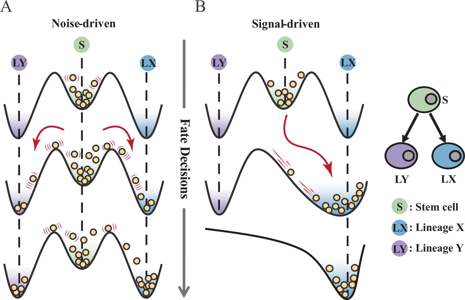
Schematic representation of cell fate decisions driven by noise (A) and signal (B) from a view of epigenetic landscape.
(A–B) Valleys represent stable attractors. Cells (yellow balls) in stem cell fate (denoted as ‘S’, green well in landscape) differentiate into downstream fates, lineage X (denoted as ‘LX’, blue well), and lineage Y (denoted as ‘LY’, purple well). These abbreviations were used for following Figures 2—7.
Figure 2
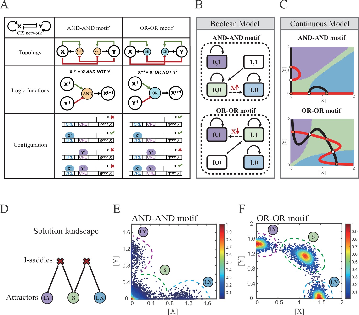
Models of the cross-inhibition with self-activation (CIS) network incorporated logic motifs.
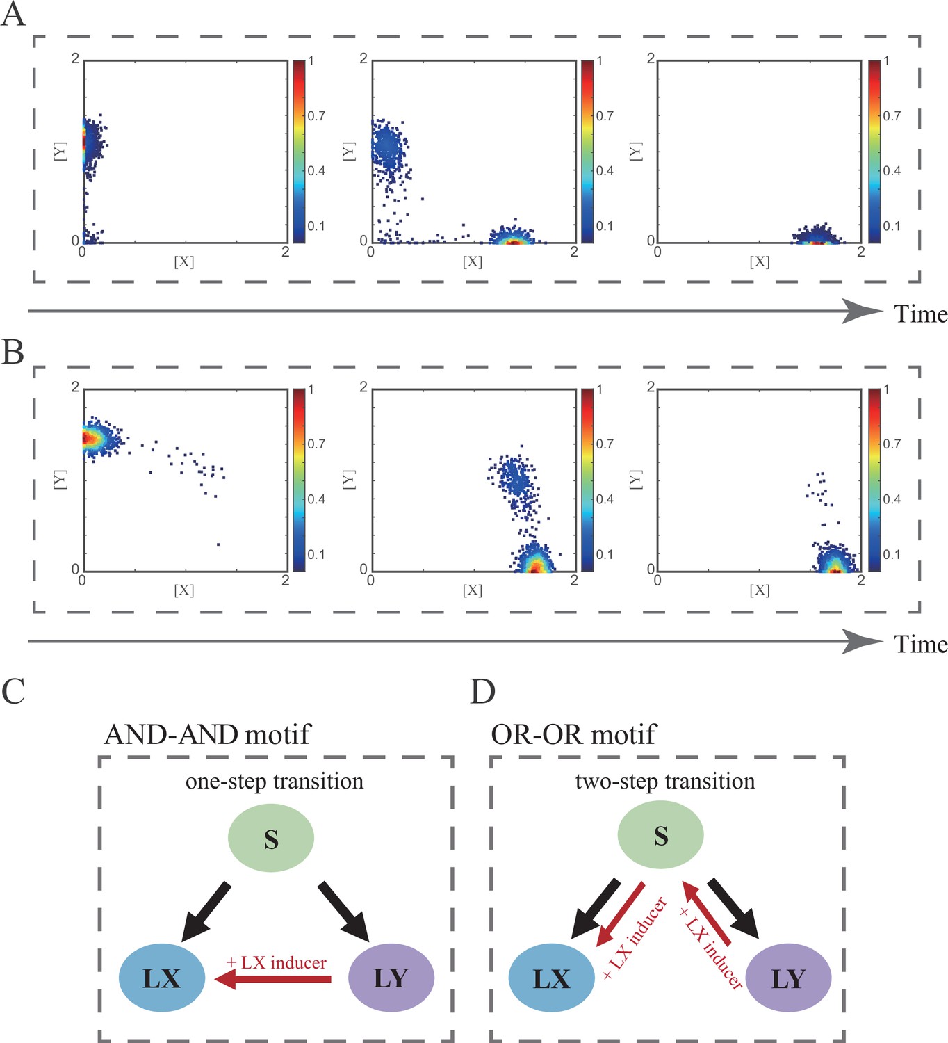
(A) A table listing the topologies with logic nodes, logic functions and Cis-regulatory elements (CRE) configurations in the CIS network incorporated AND-AND and OR-OR logic (denoted as AND-AND motif and OR-OR motif). X and Y are lineage-specifying transcription factors (TF). Xt+1 indicates the value of X at the next time step. X*, Y* represent activated forms of X and Y, respectively. The true or false signs denote whether gene X can be transcribed, respectively. These annotations were used for the following Figures 3—7. (B) State spaces of the AND-AND (top panel) and OR-OR (bottom panel) motifs in Boolean models. Updated rules of Boolean models are stated in Figure 2A. Rectangles indicate cell states. Green, blue, and purple represent S, LX, and LY, respectively. Solid arrows indicate transitions between states under corresponding Boolean models. Dotted arrows indicate forced transition imposed by external perturbations. (C) State spaces of the AND-AND (top panel) and OR-OR (bottom panel) motifs in ODE models. Dark and red lines represent nullclines of , , respectively. Stable steady states (SSS) are denoted as orange dots. Unstable steady states (USS) are denoted as white dots. Each axis represents the concentration of each transcription factor, which units are arbitrary. Blue, green, and purple areas in state spaces indicate attractor basins representing LX, S, and LY, respectively. Color of each point in state space was assigned by the attractors they finally enter according to the deterministic models (Equation 1, Equation 2). These annotations were used for the following Figures 3—7. (D) The solution landscape both for the AND-AND and OR-OR motifs. The crimson X-cross sign denotes the first-order saddle node. Blue, green, and purple circles indicate attractors. These annotations were used for the following Figures 3—7. (E–F) Simulation result of stochastic differential equation models of the AND-AND (E) and OR-OR (F) motifs. Other than adding a white noise, parameters were identical with those in (C). Initial values were set to the attractor representing S fate in Figure 2C top panel (E) and Figure 2C bottom panel (F). Noise levels of X (σx) and Y (σy) are both set to 0.14 in the AND-AND motif (E), and 0.1 in the OR-OR motif (F). Stochastic simulation was preformed 3500 times, with each final state recorded as a dot on the plot. Color of heatmap corresponds to the density of points. Unit of concentration is arbitrary.
Figure 3 with 1 supplement
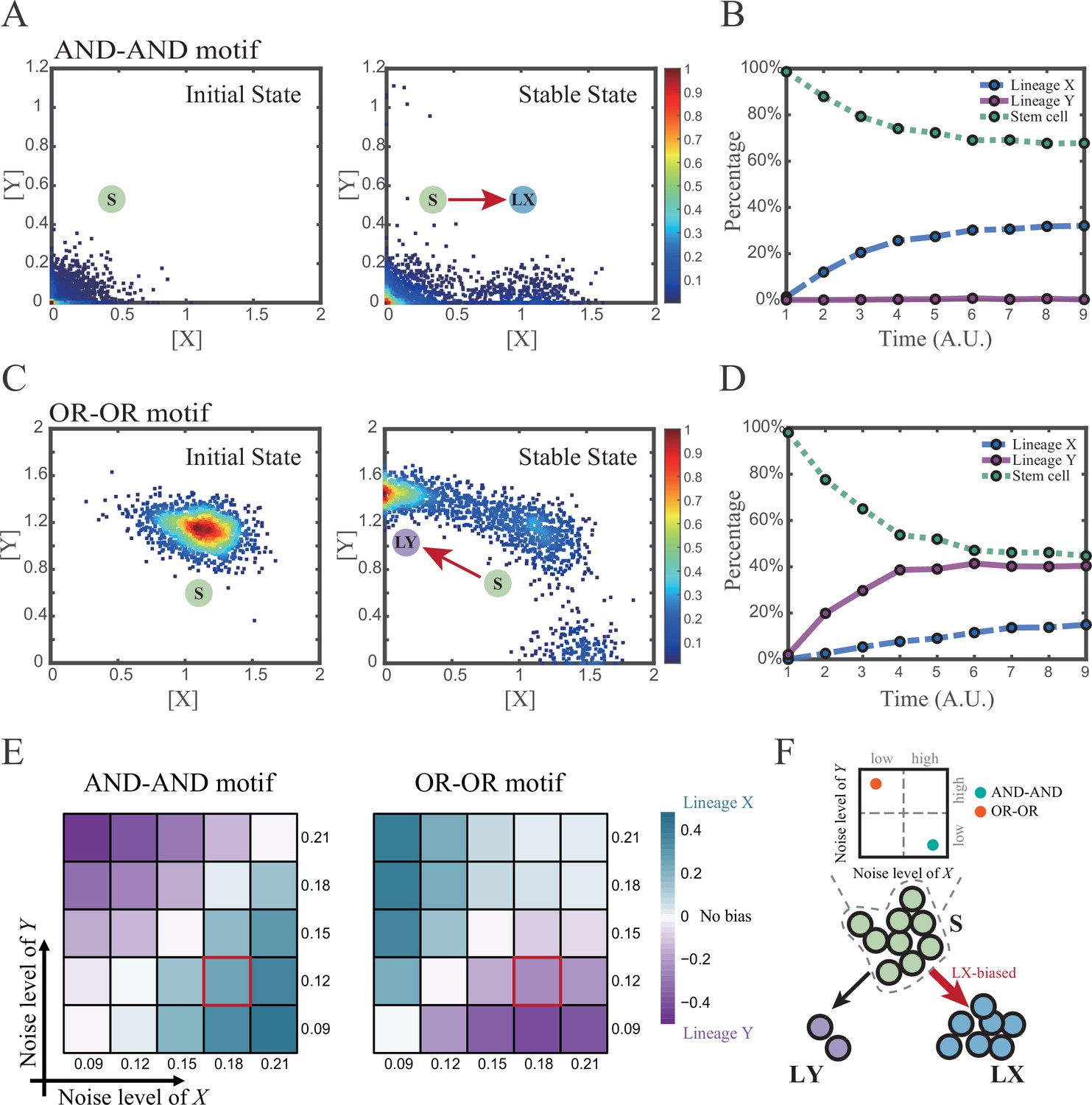
Two logic motifs exhibit opposite bias of fate decisions under the noise-driven mode.
(A and C) Stochastic simulation in both the AND-AND and OR-OR motifs. σx is set to 0.18, and σy is 0.12. In both (A) and (C), initial values were identical with attractors of stem cell fate in Figure 2C (SSSs in green attractor basins). Simulation was preformed 1500 times, with each initial (A left and C left) and final (A right and C right) states recorded as a dot on the plot. (B and D) Time courses of the percentage of cells in different fates in stochastic simulation, under the AND-AND motif (B) and OR-OR motif (D). Fates of cells were assigned by their final states according to the basins of the deterministic models in Figure 2C. Unit of time is arbitrary. (E) Heatmaps showing the bias of cell fate decisions under different noise levels of X and Y. Color of heatmap indicates the extent of bias. Here, . nLX, nLY represent number of LX, LY, respectively. ntotal represents the total number of cells (ntotal=1500). The method of assigning fate to cells is identical with Figure 3B and D. The red-marked cells correspond to the noise conditions simulated in (A) and (C). (F) Schematic illustration in that stem cell populations possessing the same bias of fate decisions need to have opposite noise patterns, according to whether they are in the AND-AND or OR-OR motif. The red and bold arrow indicates the bias of fate decisions.
Figure 3—figure supplement 1
Noise as a driving force for reprogramming of LY to S in two logic motifs.
(A) Stochastic simulation in the AND-AND motif. Initial values were identical with the attractor of LY fate in Figure 2C top panel (stable steady state, SSS in purple attractor basin). Simulation was preformed 1000 times, with each final state recorded as a dot on the plot. Top panel: Noise level of X (σx) is set to 0.03, 0.09, 0.15, from left to right, and σy is 0.03. Bottom panel: Noise level of Y (σy) is set to 0.03, 0.09, 0.15, from left to right, and σx is 0.03. Red arrow represents the direction of fate transitions of LY to S. Other than adding a white noise, parameters were identical with those in Figure 2C top panel. Color of heatmap corresponds to the density of points. (B) Stochastic simulation in the OR-OR motifs. Initial values were identical with attractor of LY fate in Figure 2C bottom panel (SSS in purple attractor basin). Simulation was preformed 1000 times, with each final state recorded as a dot on the plot. Top panel: Noise level of X (σx) is set to 0.03, 0.09, 0.15, from left to right, and σy is 0.03. Bottom panel: Noise level of Y (σy) is set to 0.03, 0.09, 0.15, from left to right, and σx is 0.03. Red arrow represents the direction of fate transitions of LY to S. Other than adding a white noise, parameters were identical with these in Figure 2C bottom panel.
Figure 4 with 1 supplement
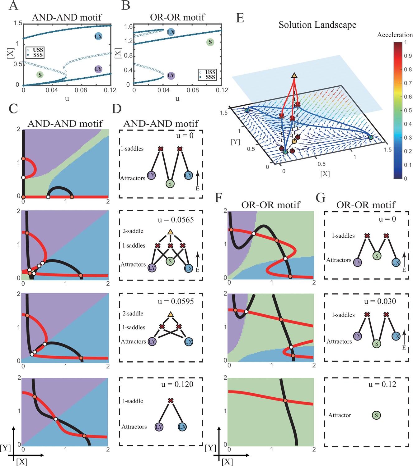
Two logic motifs decide oppositely between differentiation and maintenance under the signal-driven mode.
(A–B) Bifurcation diagrams for the AND-AND motif (A) and OR-OR motif (B) driven by parameter u (u=ux=uy) in the cross-inhibition with self activation (CIS) model. Stable steady states (SSS) and unstable steady states (USS) are denoted as solid dots and hollow dots, respectively. (C and F) Changes in the state spaces for the AND-AND motif (C) and OR-OR motif (F) with increasing parameter u, from top to down. (D and G) Changes in the solution landscape with increasing of u, in company with these in (C and F). The crimson X-cross sign and yellow triangle denote first-order and second-order saddle nodes, respectively. Relative energy is quantified by the geometric minimum action method (Vanden-Eijnden and Heymann, 2008), see ‘Materials and methods’. (E) The solution landscape with parameter u=0.0565 for the AND-AND motif from a view of three dimensions. It describes a hierarchical structure of the steady states. From top to bottom, it represents 2-saddle (yellow triangle), 1-saddles (crimson X-cross sign), and the attractors (green dot). The layer of 1-saddles is represented by a blue translucent plane, and the bottom layer is the flow field diagram. The connections from 2-saddle to 1-saddles are represented by red lines, and the connection from 1-saddles to the attractors are represented by blue lines. In the flow field diagram, the direction and color of the arrows correspond to the direction and size of the flow at that location. The corresponding positions of 2-saddle and 1-saddles in the flow field are marked with yellow and red dots, respectively, with black dashed lines indicating the corresponding relationship.
Figure 4—figure supplement 1
Two logic motifs are associated with opposite fate-decision choices under bidirectional induction.
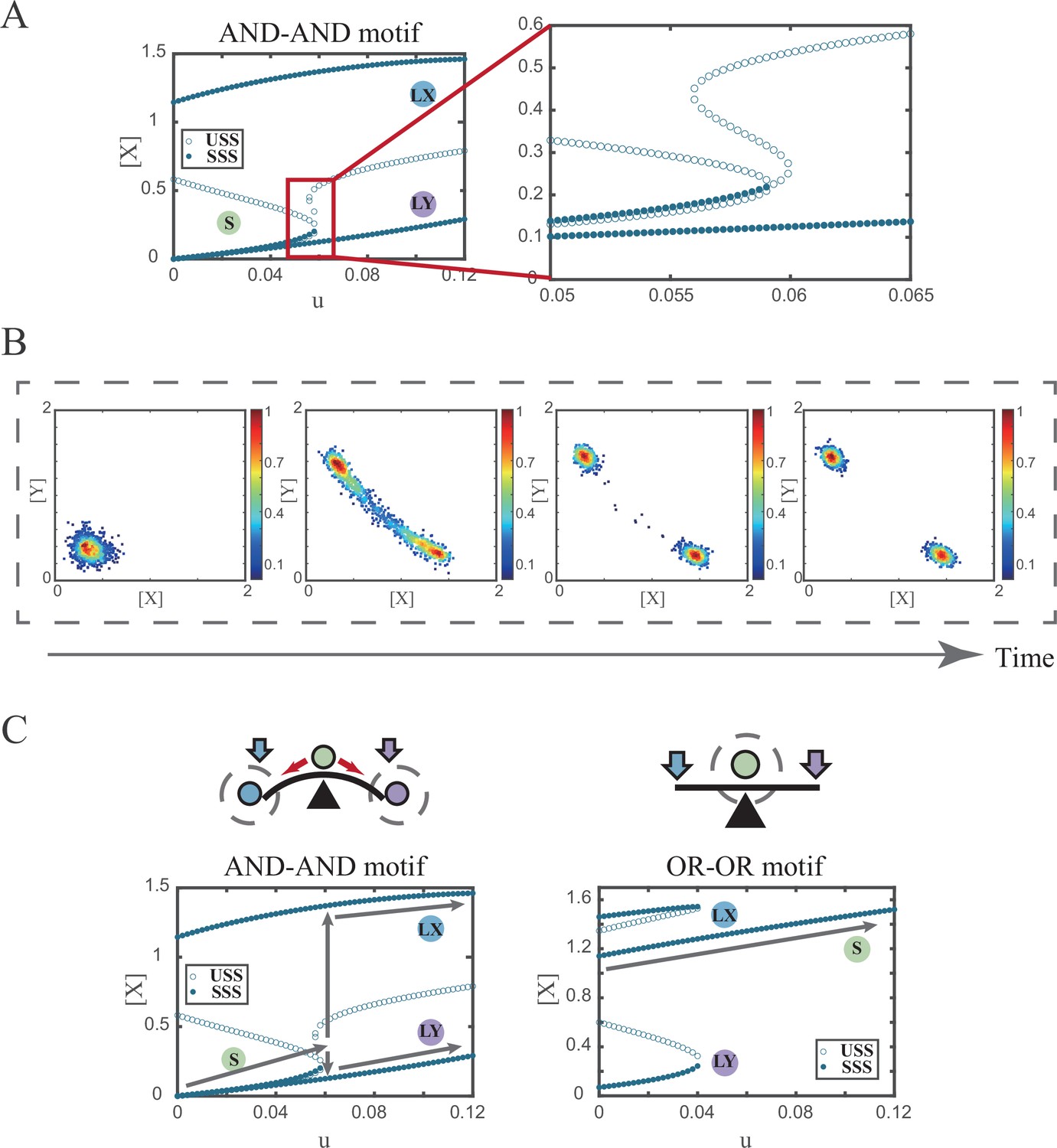
(A) Bifurcation diagrams for the AND-AND motif (Figure 4A) driven by parameter u (u=ux=uy) in the cross-inhibition with self activation (CIS) model. Stable steady states (SSS) and unstable steady states (USS) are denoted as solid dots and hollow dots, respectively. (B) Stochastic simulation in the AND-AND motif. Initial values were identical with attractor of S fate in Figure 2C top panel (SSS in green attractor basin). Noise level of X (σx) and Y (σy) are both set to 0.06. Simulation was preformed 1000 times for each pseudo-time point, with each temporal state (from left to right) recorded as a dot on the plot. Model’s parameters were identical with those in Figure 4C fourth panel. (C) Schematic illustration of the ‘seesaw’ model (Shu et al., 2013) in two logic motifs under bidirectional induction. Red arrows represent the direction of fate transitions. Blue and purple arrows represent induction of X and Y, respectively. Gray hollow circles indicate remained cell states. Gray arrows represent fate transitions from S in bifurcation diagrams as increasing u.
Figure 5 with 2 supplements
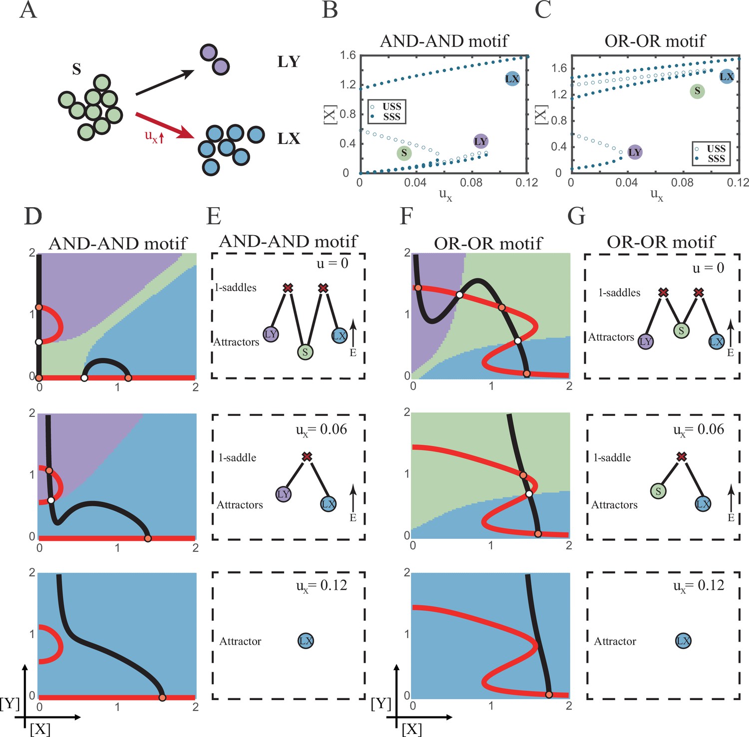
The progression-accuracy trade-off in cell fate decisions.
(A) Schematic illustration of S-to-LX cell fate decisions with X-inducing signals. The red and bold arrow indicates the direction of fate decisions. (B–C) Bifurcation diagrams for the AND-AND motif (B) and OR-OR motif (C) driven by parameter ux. (D and F) Changes in the state spaces for the AND-AND motif (D) and OR-OR motif (F) with increasing values of ux, from top to down. (E and G) Changes in the solution landscape with increasing of ux, in company with these in (D and F).
Figure 5—figure supplement 1
The PA (progression and accuracy) trade-off of cell fate decisions under the signal-driven mode.
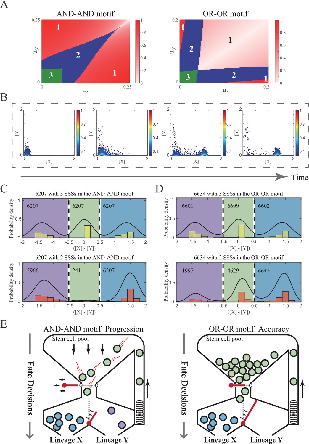
(A) Phase portraits ux vs. uy for the AND-AND and OR-OR motifs. The numbers in separating regions indicate the number of SSS. The extent of red color is quantified by minus of [X] and [Y], which indicates the expression level of balance between X and Y genes. (B) Stochastic simulation in the AND-AND motif. Initial values were identical with attractor of S fate in Figure 2C top panel (SSS in green attractor basin). Noise level of X (σx) and Y (σy) are set to 0.05, 0.15, respectively. Simulation was preformed 1000 times for each pseudo-time point, with each temporal state (from left to right) recorded as a dot on the plot. Model’s parameters were identical with those in Figure 5D middle panel. (C–D) Distribution of SSSs under all parameter sets in two logic motifs. We collected parameter sets with three SSSs, where two USSs are remained by increasing ux (see ‘Materials and methods’). Minus of [X] and [Y] of each SSS is quantified to represent relative cell fate LX, S, LY. Dark lines are kernel density estimation of each distribution. The numbers in separating regions indicate the number of SSS. (E) Schematic illustration of PA trade-off. Left panel: the entire red latch of stem cell pool is undone, which indicates all the stem cells are engaged in differentiation with fate bias (the red bar between LX and LY). Right panel: the gate for differentiating into LY is inaccessible, which indicates stem cells ‘flow’ into LX exclusively. Style was inspired by Chen et al., 2018 and Goldberg et al., 2007.
Figure 5—figure supplement 2
Distinct trajectories of reprogramming under the signal-driven mode.
(A–B) Stochastic simulation in the AND-AND (A) and OR-OR (B) motifs. Initial values were identical with attractor of LY fate in Figure 2C (SSSs in purple attractor basins). Noise level of X (σx) and Y (σy) are both set to 0.09. Simulation was preformed 1000 times, with each final state recorded as a dot on the plot. Parameter ux switched from 0 to 0.12 (0, 0.06, 0.12, from left to right). Other model’s parameters were identical with those in Figure 2C. (C–D) Schematic illustration of trajectories of reprogramming in the AND-AND (C) and OR-OR (D) motifs. Dark arrows indicate in vivo differentiation from stem cell population. Red arrows indicate trajectories of trans-differentiation under the induction of X.
Figure 6 with 2 supplements
The cross-inhibition with self activation (CIS) network performs differently during hematopoiesis and embryogenesis.
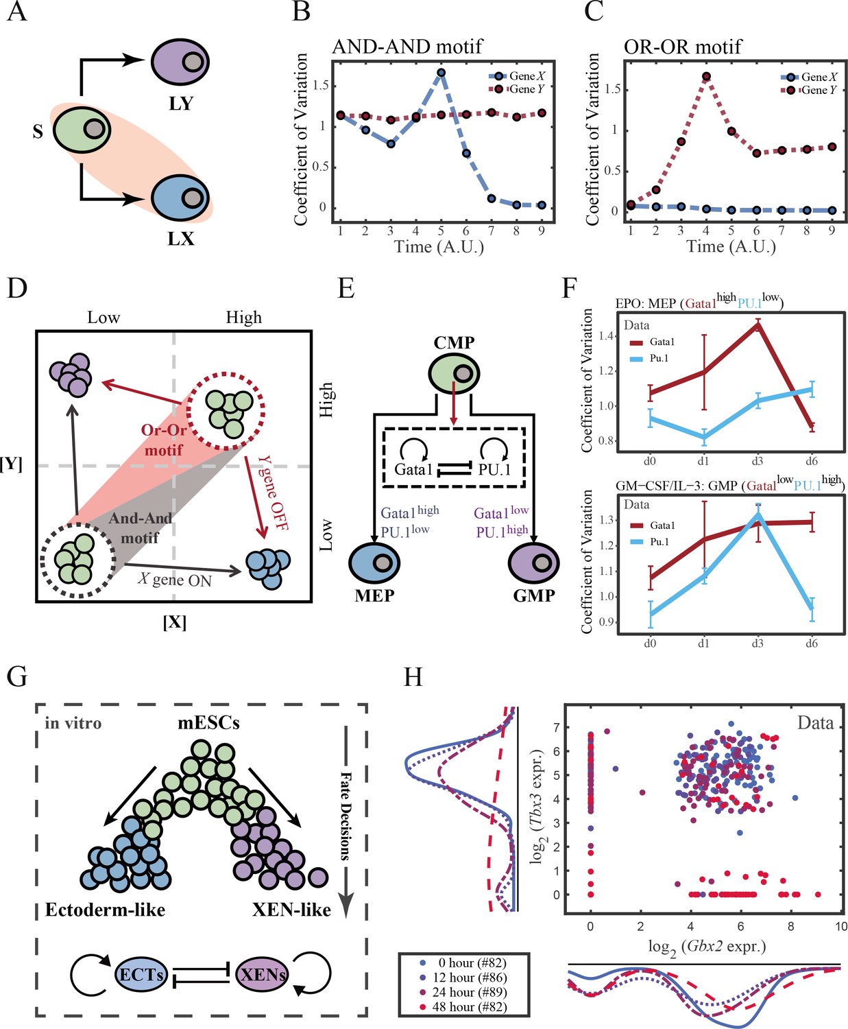
(A) Schematic illustration of S differentiating into LX. We took fate transition labeled in light pink shade as an example in the following simulation. (B) Time courses on the coefficient of variation in expression levels of X and Y genes in silico during differentiation towards LX (ux switches from 0 to 0.08 from time point 1–9) in the AND-AND motif. Initial values were set to the attractors of stem cell fate in Figure 2C top panel (SSS in green attractor basin). σx and σy are both set to 0.07. Stochastic simulation was preformed 1000 times for each pseudo-time point. Unit of time is arbitrary. (C) Time courses on the coefficient of variation in expression levels of X and Y genes in silico during differentiation towards LX (ux switches from 0 to 0.24 from time point 1–9) in the OR-OR motif. Initial values were set to the attractors of stem cell fate in Figure 2C bottom panel (stable steady state, SSS in green attractor basin). σx and σy are both set to 0.05. Stochastic simulation was preformed 1000 times for each pseudo-time point. Unit of time is arbitrary. (D) Schematic illustration of distinctive cell fate decision patterns under the AND-AND and OR-OR motifs in the state space. Dark and red gradients represent the extent of ‘AND-AND’ and ‘OR-OR’ in the actual regulatory network, respectively. Each axis represents expression levels of the lineage-specifying transcription factors. Blue, green, and purple circles indicate the cell fates of LX, S, and LY, respectively. (E) Schematic illustration of Gata1-PU.1 circuit that dominates the primary fate decisions in hematopoiesis (CMP: Common myeloid progenitor; MEP: megakaryocyte-erythroid progenitor; GMP: Granulocyte-monocyte progenitor). (F) Measured coefficient of variation of expression levels of Gata1 and PU.1 changing over time during differentiation from CMPs to MEPs and GMPs. Expression levels were quantified via single-cell RT-qPCR (Mojtahedi et al., 2016). Error bars on points represent standard deviation (SD). For details of data processing, see ‘Materials and methods’. (G) Schematic illustration of the differentiation from mESCs in an induction system (Semrau et al., 2017). (H) Measured expression levels of Gbx2 and Tbx3 among cells in embryogenesis quantified via single-cell SMART-seq2 (Semrau et al., 2017). For details of data processing, see ‘Materials and methods’.
Figure 6—figure supplement 1
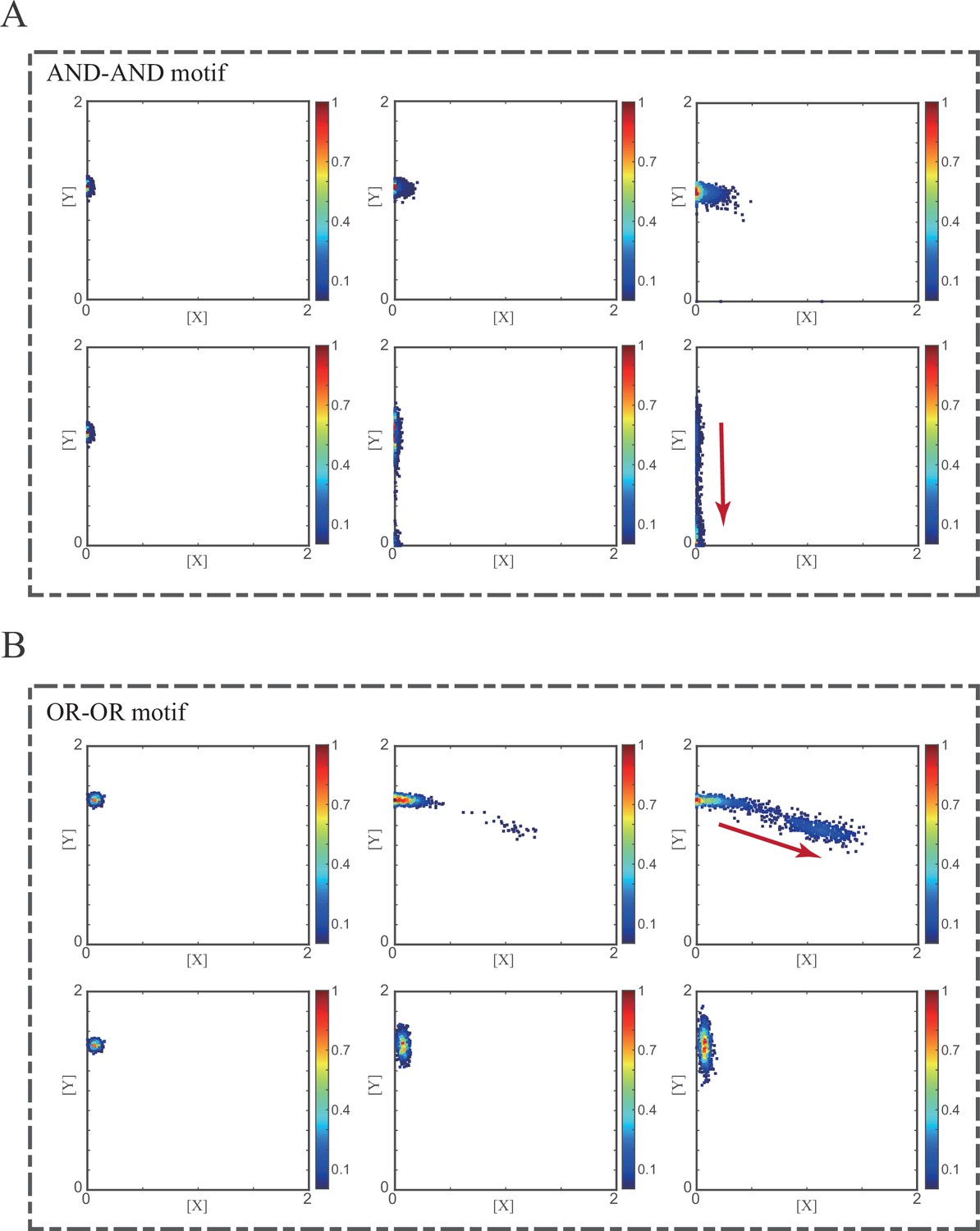
Simulation of fate transitions of S to LX in silico in two logic motifs under two driving forces.
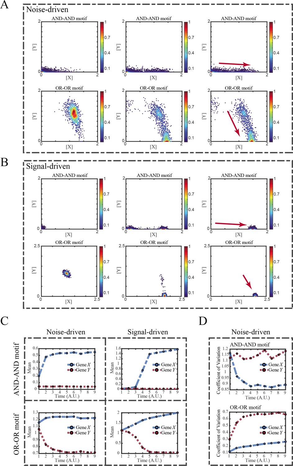
(A) Simulation in two logic motifs under the noise-driven mode. Initial values were identical with attractor of S fate in Figure 2C (Stable steady states, SSSs in green attractor basins). Simulation was preformed 1000 times for each pseudo-time point, with each temporal state (from left to right) recorded as a dot on the plot. Top panel: Noise level of X (σx) is set to 0.21, and σy is 0.09. Bottom panel: Noise level of Y (σy) is set to 0.21, and σx is 0.09. Red arrow represents the direction of fate transitions of S to LX. Other than adding a white noise, parameters were identical with those in Figure 2C. (B) Simulation in two logic motifs under the signal-driven mode. Initial values were identical with attractor of S fate in Figure 2C (SSSs in green attractor basins). Top panel: Noise level of X (σx) and Y (σy) are both set to 0.06. Simulation was preformed 1000 times, with each final state recorded as a dot on the plot. Parameter ux switched from 0 to 0.09 (0, 0.045, 0.09, from left to right). Bottom panel: Noise level of X (σx) and Y (σy) are both set to 0.05. Simulation was preformed 1000 times, with each final state recorded as a dot on the plot. Parameter ux switched from 0 to 0.24 (0, 0.12, 0.24, from left to right). Red arrow represents the direction of fate transitions of S to LX. Other model’s parameters were identical with those in Figure 2C. (C) Time courses on the mean in expression levels of X and Y genes in silico during differentiation towards LX. Initial values were set to the attractors of S fate in Figure 2C (SSSs in green attractor basins). Simulation of the noise-driven mode in two logic motifs was identical with that in Figure 6—figure supplement 1A. Simulation of the signal-driven mode in two logic motifs was identical with that in Figure 6—figure supplement 1B (Parameter ux switched from 0 to 0.12 from time point 1–9 in the AND-AND motif). (D) Time courses on the coefficient of variation in expression levels of X and Y genes in silico during differentiation towards LX under the noise-driven mode. Initial values were set to the attractors of S fate in Figure 2C (SSSs in green attractor basins). Simulation of the noise-driven mode in two logic motifs was identical with that in Figure 6—figure supplement 1A.
Figure 6—figure supplement 2
Gene regulatory networks (GRNs) perform differently in differentiations during hematopoiesis and embryogenesis.
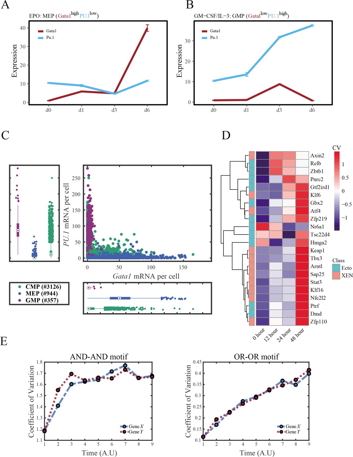
(A–B) Measured mean of expression levels of Gata1 and PU.1 changing over time in the processes of differentiation from Common myeloid progenitors (CMP) to megakaryocyte-erythroid progenitors (MEP) and Granulocyte-monocyte progenitors (GMP). Expression levels were quantified via single-cell RT-qPCR (Mojtahedi et al., 2016). For details of data processing, see ‘Materials and methods. (C) Expression level of Gata1 and PU.1 among CMPs, MEPs, and GMPs quantified via single-molecule RNA fluorescent in situ hybridization (Wheat et al., 2020). (D) Heatmap of coefficient of variation of expression levels of 22 genes among cells in embryogenesis quantified via single-cell SMART-seq2 (Semrau et al., 2017). For details of data processing, see ‘Materials and methods’. (E) Time courses on the coefficient of variation in expression levels of X and Y genes in silico during differentiation under the noise-driven mode. Initial values were set to the attractors of S fate in Figure 2C (Stable steady states, SSSs in green attractor basins). Top panel: Noise level of X (σx) and Y (σy) are both set to 0.14. Bottom panel: Noise level of X (σx) and Y (σy) are both set to 0.1. Stochastic simulation was preformed 1000 times for each pseudo-time point.
Figure 7 with 1 supplement
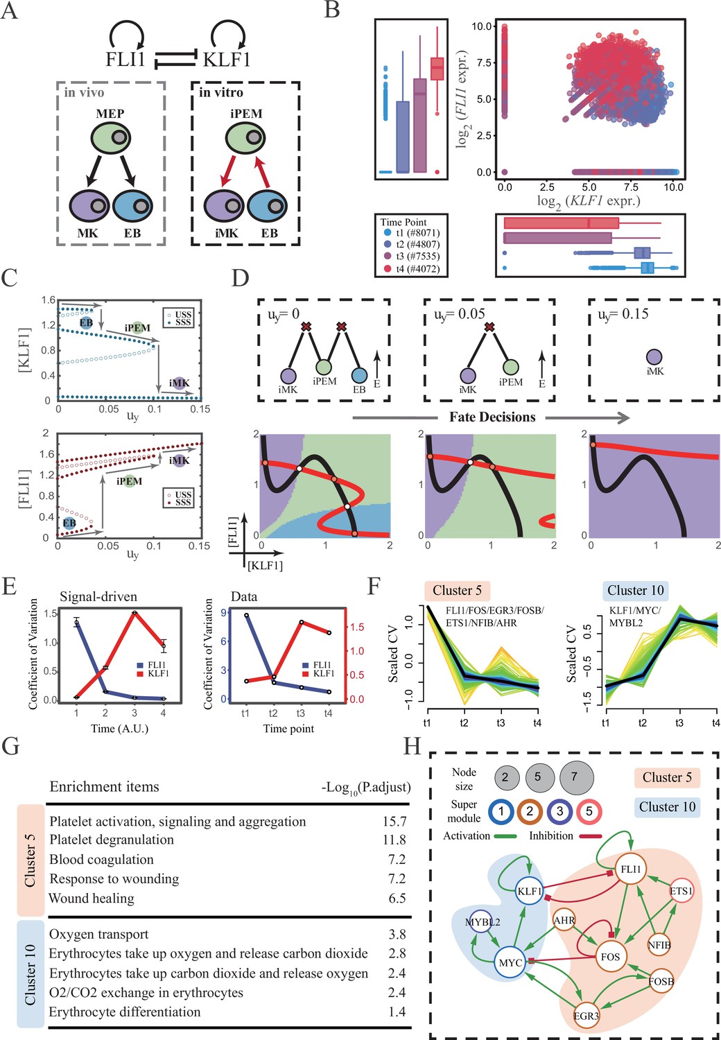
The chemical-induced reprogramming of human erythroblast (EB) to induced megakaryocyte (iMK) is the signal-driven fate decisions with an OR-OR-like motif.
(A) Schematic illustration of the differentiation from megakaryocyte-erythroid progenitors (MEPs) in vivo and in vitro.Red arrows represent the route of reprogramming (Qin et al., 2022) (B) Measured expression levels of KLF1 and FLI1 in reprogramming quantified via single-cell 10 X. For details of data processing, see ‘Materials and methods’. (C) Bifurcation diagrams for the OR-OR motif driven by parameter uy in the CIS model. (D) Fate transition representing reprogramming of EB to iMK in silico. Top panel: changes in the solution landscape with increasing of parameter uy, from left to right; Bottom panel: changes in the state spaces for the OR-OR motif with increasing values of uy, in company with these in top panel. Unit of concentration is arbitrary. (E) Left panel: coefficient of variation of expression levels of KLF1 and FLI1 changes in silico over time under given parameter (uy=0.11) in the OR-OR motif. Noise level of KLF1 (σx) and FLI1 (σy) are set to 0.087. Initial values were identical with LX attractor in Figure 2C bottom panel (stable steady state, SSS in blue attractor basin). Stochastic simulation was preformed 1000 times per round for each time point. We totally preformed three round simulations. Error bars on points represent standard deviation (SD); Right panel: measured coefficient of variation of expression levels of KLF1 and FLI1 changing over time in the processes from EBs to iMKs. Unit of time is arbitrary. (F) Identification of distinct temporal patterns of expression variance by fuzzy c-means clustering. The x-axis represents four time points, while the y-axis represents scaled CV (coefficient of variation) in each time point. Dark trend lines in the middle indicate the average of scaled CV over genes in cluster. (G) Enriched major Gene Ontology terms for clusters 5 and 10. (H) Regulatory network of transcription factors (TFs) in cluster 5 and 10. Circle size indicates the sum of in-degree and out-degree. Node colors indicate different Supermodules (adapted from Qin et al., 2022). Green and red edges indicate activation and inhibition, respectively. The light blue and light pink shades denote genes in clusters 5 and 10, respectively.
Figure 7—figure supplement 1

The chemical-induced reprogramming of human erythroblast (EB) to induced megakaryocyte (iMK) is the signal-driven fate decisions.
(A) Time courses on the mean in expression levels of KLF1 and FLI1 genes in silico during reprogramming of EBs to iMKs under the noise-driven (left) and signal-driven (right) modes. Initial values were set to the attractors of LX fate in Figure 2C bottom panel (SSS in blue attractor basin). Noise level of KLF1 (σx) and FLI1 (σy) are both set to 0.18 under the noise-driven mode. Stochastic simulation was preformed 1000 times for each pseudo-time point. Other than adding a white noise, parameters were identical with those in Figure 2C bottom panel. Simulation of the signal-driven mode was identical with that in Figure 7E left panel. (B) Coefficient of variation of expression levels of KLF1 and FLI1 changes in silico along by pseudo-time under the OR-OR motif. Simulation was identical with that in Figure 7—figure supplement 1 left panel. (C) Identification of distinct temporal patterns of expression variance by fuzzy c-means clustering. The x-axis represents four time points, while the y-axis represents scaled CV (coefficient of variation) in each time point. Dark trend lines in the middle indicate average of scaled CV over genes in cluster.
Author response image 1

Initial values were identical with attractor of S fate in Figure 2C (SSSs in green attractor basins).
Simulation was preformed 1000 times for each pseudo-time point, with each temporal state (from left to right) recorded as a dot on the plot. Top panel: Noise level of X (σx) is set to 0.21, and σy is 0.09. Bottom panel: Noise level of Y (σy) is set to 0.21, and σx is 0.09. Red arrow represents the direction of fate transitions of S to LX. Other than adding a white noise, parameters were identical with those in Figure 2C.”
Author response image 2

Initial values were identical with attractor of S fate in Figure 2C (SSSs in green attractor basins).
Top panel: Noise level of X (σx) and Y (σy) are both set to 0.06. Simulation was preformed 1000 times, with each final state recorded as a dot on the plot. Parameter ux switched from 0 to 0.09 (0, 0.045, 0.09, from left to right). Bottom panel: Noise level of X (σx) and Y (σy) are both set to 0.05. Simulation was preformed 1000 times, with each final state recorded as a dot on the plot. Parameter ux switched from 0 to 0.24 (0, 0.12, 0.24, from left to right). Red arrow represents the direction of fate transitions of S to LX. Other model’s parameters were identical with those in Figure 2C.”
Author response image 3

Additional files
-
Supplementary file 1
Parameter sets for screening fully-connected stage in two logic motis.
The spreadsheet titled ‘MAP’ gives the relative energy in Figure 4D and G, Figure 5E and G, Figure 7D.
- https://cdn.elifesciences.org/articles/88742/elife-88742-supp1-v1.xlsx
-
Supplementary file 2
1677 TFs divided into 12 clusters based on time-course CV.
The spreadsheet lists all 12 clusters of TFs, as described in Figure 7F, Figure 7—figure supplement 1C.
- https://cdn.elifesciences.org/articles/88742/elife-88742-supp2-v1.xlsx
-
Supplementary file 3
Integrated human TF list and regulon database.
The spreadsheet records the human TF list and regulon used in Figure 7H.
- https://cdn.elifesciences.org/articles/88742/elife-88742-supp3-v1.xlsx
-
MDAR checklist
- https://cdn.elifesciences.org/articles/88742/elife-88742-mdarchecklist1-v1.docx
Download links
A two-part list of links to download the article, or parts of the article, in various formats.
Downloads (link to download the article as PDF)
Open citations (links to open the citations from this article in various online reference manager services)
Cite this article (links to download the citations from this article in formats compatible with various reference manager tools)
A logic-incorporated gene regulatory network deciphers principles in cell fate decisions
eLife 12:RP88742.
https://doi.org/10.7554/eLife.88742.3


