Functional imaging of conduction dynamics in cortical and spinal axons
- Uppsala University, Department of Medical Sciences, Sweden
Figures
Figure 1 with 2 supplements

Reconstruction of axonal morphology based on neuronal electrical activity.
(A) Contour map shows spatial distribution of extracellular action potentials (APs) recorded from a single cortical neuron. Average AP amplitudes are color-coded and presented through contour surfaces. Gray dots in the background represent locations of the recording electrodes. White-dashed-line circles superimposed over the contour map denote three magnified regions displayed on the right. Average AP waveforms obtained from proximal, middle, and distal axons are shown in the three denoted regions (labeled I, II, and III, respectively); color-coding is the same as in the contour map. Examples of AP waveforms recorded from the axon initial segment (AIS) and distal axons are shown at the bottom. (B) Functional morphology of axonal arbor reconstructed from APs displayed in (A). Branching orders of reconstructed neurites are color-coded. The AIS is depicted by a thick red line superimposed over the most proximal part of the axon. A filled dark-brown circle represents putative location of the neuronal soma. Color-free contour map and recording electrodes are shown in the background (same as in A). Functional morphologies of cortical and spinal axons are also presented in Figure 1—videos 1 and 2, respectively.
Figure 1—video 1
Functional morphologies of cortical axons displayed in real time.
(Left) Reconstructed functional morphologies of cortical axons superimposed over a micrograph of the corresponding culture. Morphologies of individual neurons are presented through consecutive sequences of action potential (AP) propagation paths as traced across axonal arbors in real time. Functional morphologies of 15 neurons are displayed successively and stacked on top of each other; neuron count is color-coded; total length of reconstructed axons amounts 348.82 mm. A micrograph of immunostained rat’s primary cortical culture grown directly on the high-density microelectrode array (HD-MEA) surface is shown in the background. The culture was fixed immediately after the acquisition of electrophysiological data, and fluorescently labeled against β-III tubulin at 16 days in vitro (DIV). Epifluorescence microscopy was used to collect optical data. (Right) Spontaneous electrical activities of cortical neurons as monitored across an entire HD-MEA. Amplitudes of electrical signals recorded by individual electrodes are color-coded in gray scale; recorded signals are mapped spatially across all microelectrodes and temporally over discrete timeframes to produce the movie. Trajectories of axonal signals are traced over consecutive timeframes to reconstruct morphologies of individual neurons. Time gap between consecutive timeframes is 50 μs. Real conduction times of traced signals are color-coded and presented through reconstructed morphologies (blue-cyan scale). Functional morphologies of 15 neurons are traced successively and simultaneously shown on both right and left panel.
Figure 1—video 2
Functional morphologies of spinal axons displayed in real time.
(Left) Reconstructed functional morphologies of motor neuron axons superimposed over a micrograph of the corresponding culture. Morphologies of individual neurons are presented through consecutive sequences of action potential (AP) propagation paths as traced across axonal arbors in real time. Functional morphologies of 15 neurons are displayed successively and stacked atop each other; neuron count is color-coded; total length of reconstructed axons amounts 282.72 mm. Micrograph of immunostained rat’s primary motor neuron culture grown directly on the high-density microelectrode array (HD-MEA) surface is shown in the background. The culture was fixed immediately after the acquisition of electrophysiological data, and fluorescently labeled against β-III tubulin at 12 days in vitro (DIV). Epifluorescence microscopy was used to collect optical data. (Right) Spontaneous electrical activities of motor neurons as monitored across an entire HD-MEA. Amplitudes of electrical signals recorded by individual electrodes are color-coded in gray scale; recorded signals are mapped spatially across all microelectrodes and temporally over discrete timeframes to produce the movie. Trajectories of axonal signals are traced over consecutive timeframes to reconstruct morphologies of individual neurons. Time gap between consecutive timeframes is 50 μs. Real conduction times of traced signals are color-coded and presented through reconstructed morphologies (blue-cyan scale). Functional morphologies of 15 neurons are traced successively and simultaneously shown on both right and left panel.
Figure 2 with 10 supplements
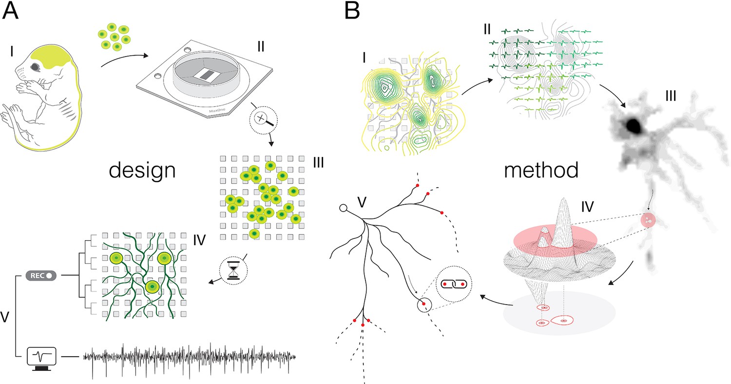
Experimental design and overview of the method.
(A) Experimental design: (I) Brain cortices and spinal cords isolated (lime-green) from Sprague Dawley rat embryos were used as sources of primary cortical and motor neurons. Cells obtained from corresponding sources were seeded directly on high-density microelectrode arrays (HD-MEAs) to grow cortical and motor neurons in separate cultures. (II) The utilized HD-MEA system features 26,400 microelectrodes packed within an area of 3.85×2.1 mm2. Interelectrode distances of 17.5 μm provide density of 3264 microelectrodes per mm2. (III) The HD-MEA surface coated with cell-adhesive materials promoted neuronal growth over the sensing area and provided efficient electrode-to-neuron contacts. (IV) Dedicated media and growth-promoting factors were used to develop and maintain the cultures in vitro over extended periods of time. (V) Mature cultures conveyed spontaneous electrical activities. Neuronal extracellular action potentials (APs) were recorded through HD-MEA recording channels at 20 kHz sampling rate. (B) Overview of the method: (I) Signal amplitudes sampled across an entire HD-MEA were used to produce network-wide activity maps (yellow-green contour map). Local peaks found in activity maps indicated locations of individual neurons in the network. (II) Spike-sorting of recorded signals enabled to discern activities between neighboring neurons and to extract their individual electrical profiles. Displayed electrical profiles (dark-, mint-, and lime-green waveforms) are referred to as ‘extracellular AP footprints’. (III) Array-wide spike-triggered averaging revealed spatiotemporal distribution of APs across axons of individual neurons (gray-scale signal map). Such representation of neuronal signals is referred to as an ‘axonal electrical image’. (IV) Dynamic thresholding was used to detect local peaks within the footprint. (V) Detected peaks were interlinked based on their spatial and temporal proximities to reconstruct axonal conduction trajectories.
Figure 2—figure supplement 1
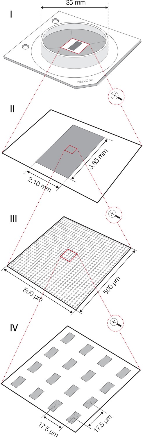
Complementary-metal-oxide-semiconductor (CMOS)-based high-density microelectrode array (HD-MEA).
Graphical scheme shows technical features of CMOS-based HD-MEA system that was used in this study. (I) Outlook of HD-MEA chip. (II) The MEA comprises 26,400 platinum electrodes packed within sensing area of ~8 mm2. Each of the electrodes can serve as a recording and/or stimulation source enabling bi-directional communication with any cell laying on the sensing area. (III) Dense arrangement of microelectrodes (3264 electrodes per mm2) enables to access electrical activity of a single neuron across hundreds of sites at subcellular spatial resolution. (IV) Sizes of individual microelectrodes are 9.3×5.45 μm2; interelectrode center-to-center pitch is 17.5 μm. Up to 1024 readout channels can be simultaneously used to sample neuronal signals. Flexible switch matrix technology allows to route available channels to desired electrodes and to reconfigure the routing within few microseconds. Raw neuronal signals are recorded at 20 kHz sampling rate.
Figure 2—figure supplement 2
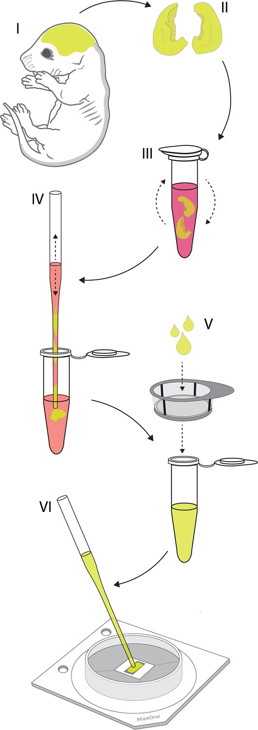
Culturing primary cortical neurons on the high-density microelectrode array (HD-MEA).
Graphical illustration shows the key steps of the protocol used for culturing rat’s primary cortical neurons on the HD-MEA surface. (I) Entire brains were obtained from Sprague Dawley rat embryos dissected on embryonic day 18. (II) Cortices were isolated from the brains and cortical meninges were removed. (III) Cortices were dissociated enzymatically in trypsin supplemented with 0.25% EDTA. (IV) Cortices were dissociated physically by trituration in the plating medium. (V) Suspension of dissociated cells was filtered using 40 µm cell strainer to remove cell aggregates and debris. (VI) Filtered cells were plated directly on the chip’s sensing area coated by a thin layer of laminin. Cells were seeded in a 20 µl drop containing ~50,000 cells in total.
Figure 2—figure supplement 3
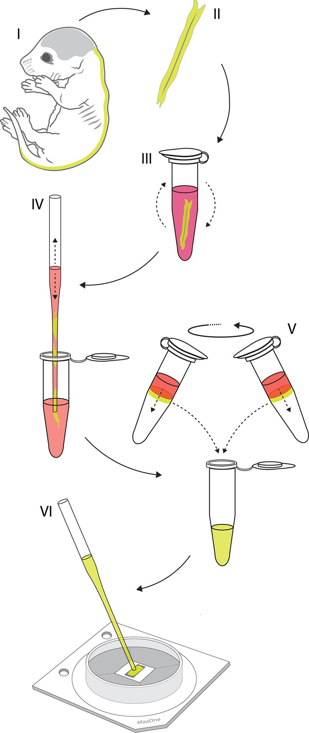
Culturing primary motor neurons on the high-density microelectrode array (HD-MEA).
Graphical illustration shows key steps of the protocol used for culturing rat’s primary motor neurons on HD-MEA surface. (I) Entire spinal cords were isolated from Sprague Dawley rat embryos dissected on embryonic day 14. (II) Dorsal root ganglia were detached and meninges were removed from isolated spinal cords. (III) Spinal cords were dissociated enzymatically in trypsin supplemented with 0.25% EDTA. (IV) Spinal cords were next dissociated physically by trituration in the plating medium. Suspension of dissociated cells was filtered using 40 µm cell strainer to remove cell aggregates and debris. (V) Density gradient centrifugation was used to fractionate motor neurons from the filtered cell suspension. (VI) Isolated cells were plated directly on the chip’s sensing area coated by a thin layer of laminin. Cells were seeded in a 20 µl drop containing ~50,000 cells in total.
Figure 2—figure supplement 4
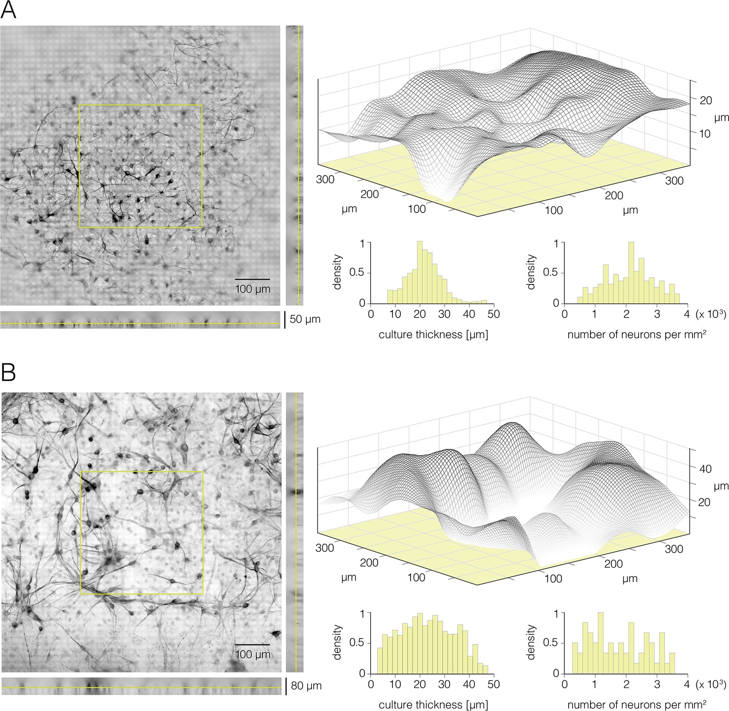
Thickness and cell density of neuronal cultures grown on the high-density microelectrode array (HD-MEA).
(A) Rat primary cortical culture grown on the HD-MEA surface – 16 days in vitro (DIV). (Left) Micrograph of the cortical culture immunostained against β-III tubulin. Epifluorescence microscopy was used to collect Z-stack image series. Z-position of the focus plane shown is marked on the side view projections (yellow lines). Yellow square superimposed over the center of the micrograph denotes a section of the Z-stack data that was used to produce the graph shown on the right. (Right) Surface plot reconstructed from the Z-stack data denoted in the left panel. Three-dimensional graph (gray net) displays intensities of fluorescent signals. Reconstructed graph was used to estimate thickness of the culture. Distribution of local thicknesses and cell densities sampled over discrete areas of 100×100 μm2 are presented in the histograms bellow. (B) Rat’s primary motor neuron culture grown on HD-MEA surface – 12 DIV. (Left) Micrograph of the motor neuron culture immunostained against β-III tubulin. Epifluorescence microscopy was used to collect Z-stack image series. Z-position of the focus plane shown is marked on the side view projections (yellow lines). Yellow square superimposed over the center of the micrograph denotes a section of the Z-stack data that was used to produce the graph shown on the right. (Right) Surface plot reconstructed from the Z-stack data denoted in the left panel. Three-dimensional graph (gray net) displays intensities of fluorescent signals. Reconstructed graph was used to estimate thickness of the culture. Distribution of local thicknesses and cell densities sampled over discrete areas of 100×100 μm2 are presented in two histograms below.
Figure 2—figure supplement 5
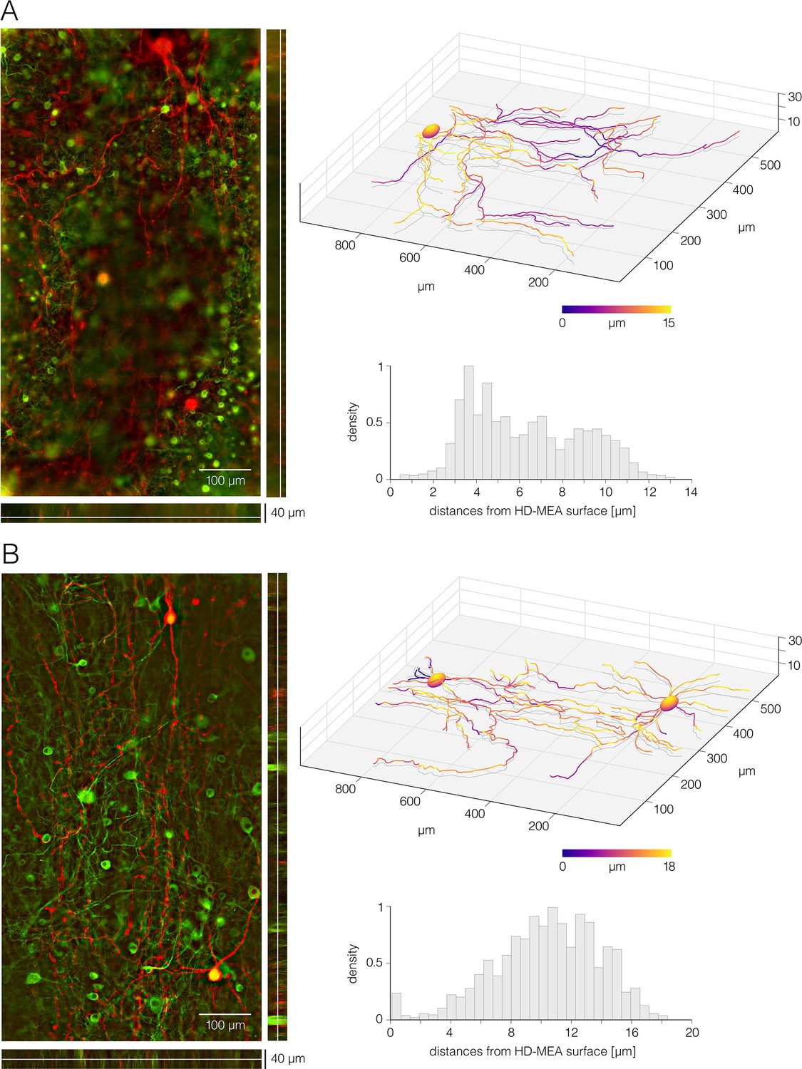
Disposition of cortical and spinal neurites with respect to the high-density microelectrode array (HD-MEA) surface.
(A) Cortical neurons grown on the HD-MEA surface – 16 days in vitro (DIV). (Left) Micrograph of fluorescently labeled cortical neurons. Neurons were sparsely transfected at 14 DIV using RFP-expressing plasmid (pAAV-hSyn-mCherry); the RFP expression was optically confirmed in six neurons. The culture was fixed at 16 DIV and immunostained against β-III tubulin to label all neurons in the culture (green); the culture was also immunostained against RFP to intensify fluorescent signal in the transfected neurons (red). Epifluorescence microscopy was used to collect Z-stack image series. (Right-up) Three-dimensional neuronal morphology reconstructed from optical data shown in the left panel. Local distances of neuronal processes from the HD-MEA surface are color-coded. (Right-down) Histogram shows distribution of local distances of neuronal processes from the HD-MEA surface. (B) Motor neurons grown on the HD-MEA surface – 12 DIV. (Left) Micrograph of fluorescently labeled motor neurons. Individual neurons were sparsely transfected at 10 DIV using RFP-expressing plasmid (pAAV-hSyn-mCherry); the RFP expression was optically confirmed in 14 neurons. The culture was fixed at 12 DIV and immunostained against β-III tubulin to label all neurons in the culture (green); the culture was also immunostained against RFP to intensify fluorescent signal in the transfected neurons (red). Epifluorescence microscopy was used to collect Z-stack image series. (Right-up) Three-dimensional neuronal morphologies reconstructed from optical data shown in the left panel. Local distances of neuronal processes from the HD-MEA surface are color-coded. (Right-down) Histogram shows distribution of local distances of neuronal processes from the HD-MEA surface. ImageJ and Matlab custom-designed codes were used to reconstruct three-dimensional neuronal morphologies shown here.
Figure 2—figure supplement 6
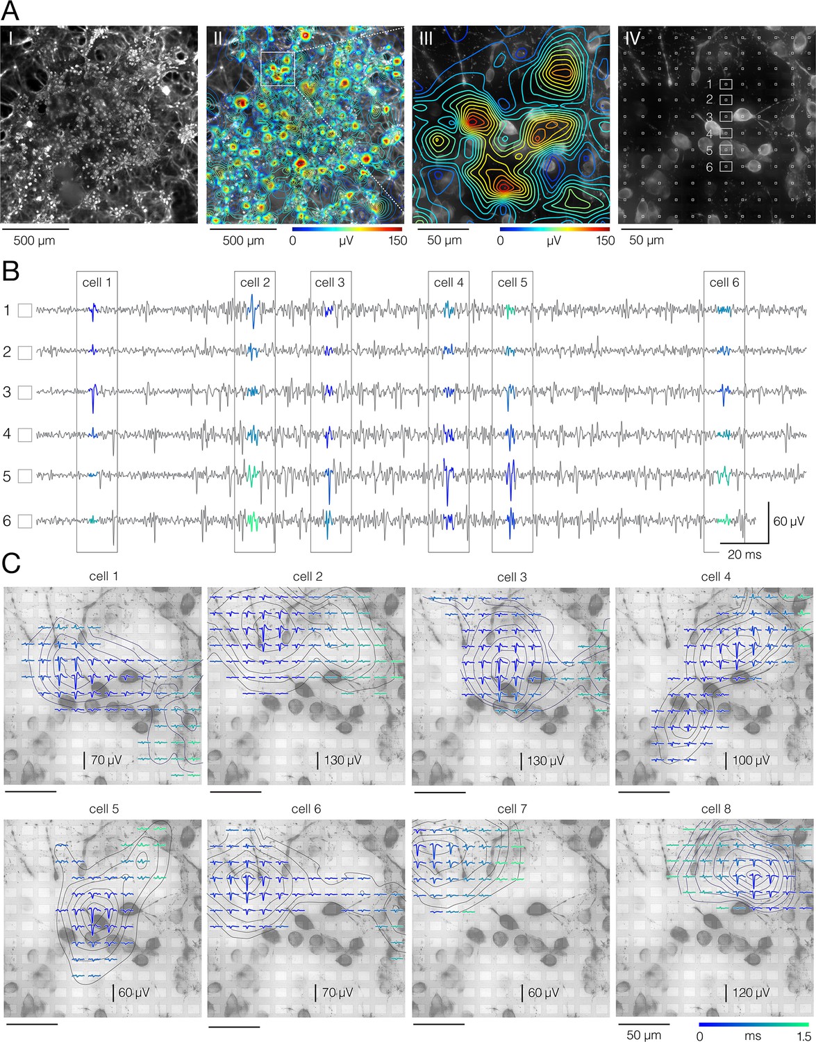
Electrical identification of individual neurons in the culture.
(A) Network-wide electrical activity. (I) Micrograph of fluorescently labeled cortical culture grown on the high-density microelectrode array (HD-MEA). The culture was fixed at 16 days in vitro (DIV) and immunostained against Map2. Epifluorescence microscopy was used to collect Z-stack image series (presented in Figure 2—video 1). Herein, presented is maximum signal intensity. (II) Network-wide activity map. Spontaneous action potentials (APs) were sampled across all microelectrodes for 2 min. Average amplitudes of recorded signals were used to reconstruct the map; signal amplitude is color-coded. Micrograph of the corresponding culture is set in back. White square superimposed over the map frames the region magnified in III. (IV) Positions of the recording microelectrodes (white squares in front) with respect to locations of neuronal somas (micrograph in the background); same region as in III; Z-stack image series are presented in Figure 2—video 2. Voltage traces recorded from six denoted electrodes (1–6) are shown in (B). (B) Discerning between APs recorded from neighboring neurons. Spike-sorting algorithms enable discerning mixed signals recorded from neighboring neurons and thereby extracting APs arising from individual neurons. Voltage traces recorded from six electrodes (denoted in A-IV) are presented in gray. Sorted signals from different cells (1–6) are colored. (C) Reconstructed electrical activities of individual neurons. Averaging of sorted signals over adjacent electrodes reveals the spatiotemporal distribution of a single neuron’s activity. Such signal representation is called an ‘extracellular AP footprint’. Herein, presented are electrical footprints of eight neighboring neurons, superimposed over micrograph of the corresponding culture (same as in A-IV). Temporal distribution of APs detected on different electrodes is color-coded.
Figure 2—figure supplement 7
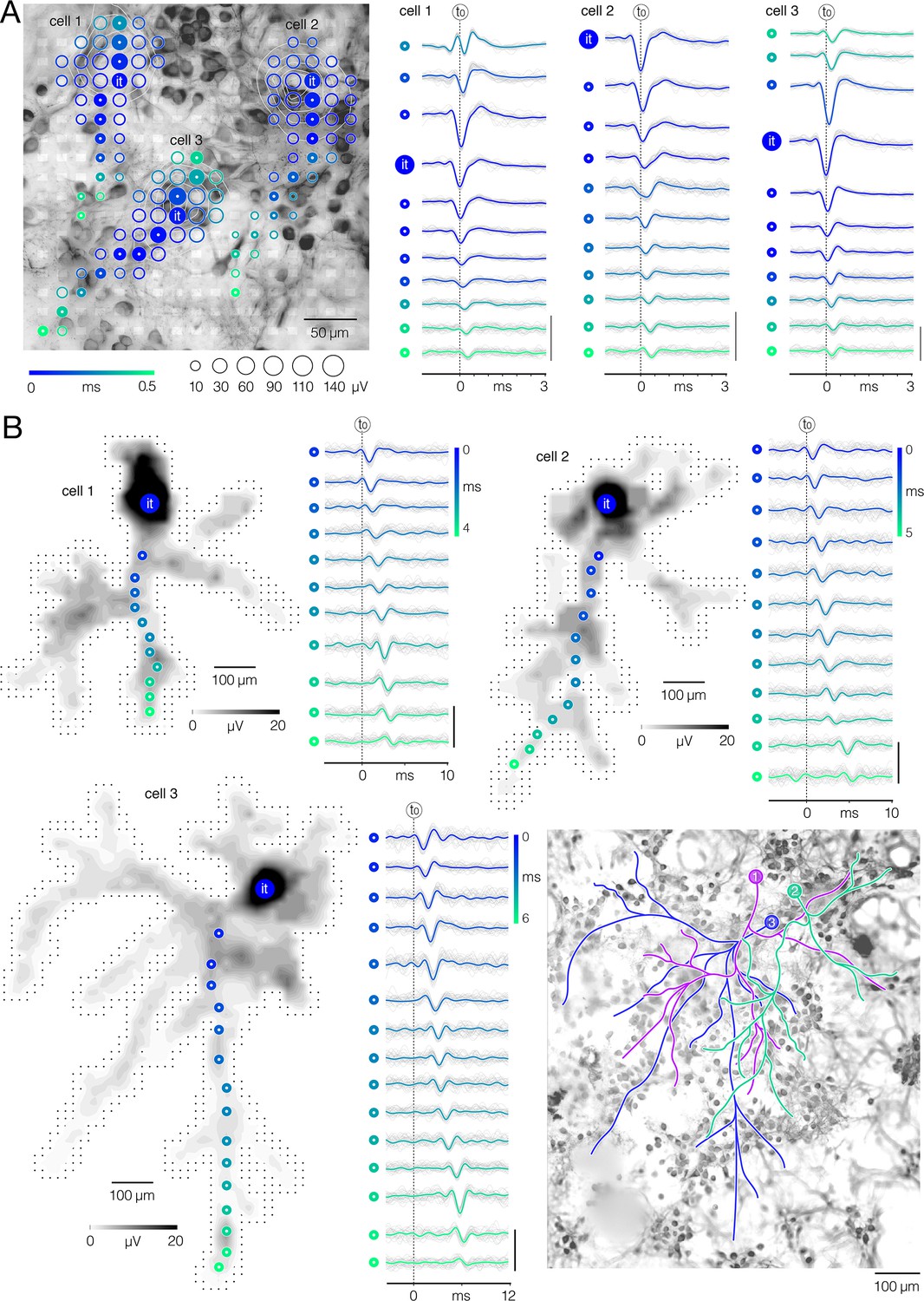
Electrical imaging of axonal arbors.
(A) Electrical footprints reveal proximal neuronal compartments. (Left) Electrical footprints of three neighboring cortical neurons (denoted as cell 1–3). Circle sizes indicate average amplitudes of action potentials (APs) detected on individual microelectrodes; occurrence time of detected AP peaks relative to timing of the initial trace (t0) is color-coded. Color-filled circles denote locations along putative dendrite-axon initial segment (AIS)-axon axis; APs recorded from the denoted locations are shown in right. Micrograph of the corresponding culture is shown in the back; the culture was fixed at 16 days in vitro (DIV) and immunostained against Map2. White semitransparent rectangles superimposed over the micrograph represent microelectrodes. (Right) AP waveforms recorded along dendrite-AIS-axon axis as denoted in left. AP waveforms are temporally aligned with respect to occurrence time of the initial trace (it); note temporal shift of the aligned AP peaks relative to t0 (black-dashed line in the back). Average AP waveforms are colored (blue-cyan) and superimposed over the corresponding single trials (gray). Color-coding same as in left. Signal scalebar: 100 μV. (B) Spike-trigger averaging of sorted APs reveals entire axonal arbors. (Left-up, Right-up, Left-down) Spatial distribution of axonal APs recorded across an entire high-density microelectrode array (HD-MEA); same neurons as in (A); AP amplitude is color-coded (gray scale). It – initial trace; color-filled circles denote recording sites for axonal APs shown on the side. Black dots in the background represent microelectrodes. Axonal AP waveforms recorded from the denoted sites are presented on the side; their occurrence time is color-coded. Average AP waveforms are colored (blue-cyan) and superimposed over the corresponding single trials (gray). Signal scalebar: 100 μV. (Right-down) Axonal contours of the three cortical neurons (denoted as 1–3) superimposed over the micrograph of the corresponding culture. Spike-trigger averaged signals of the three neurons are presented in Figure 2—video 3. Axonal contours are estimated by observing spatial movements of the signal peaks in consecutive movie frames. The culture was fixed at 16 DIV and immunostained against Map2. Epifluorescence microscopy was used to collect Z-stack image series (presented in Figure 2—video 1).
Figure 2—video 1
Cortical culture grown on high-density microelectrode array (HD-MEA) surface – ×20 magnification.
Z-stack image series of cortical culture grown on the HD-MEA. The presented culture section covered an area of 1.3×1.3 mm2 and interfaced with 5476 electrodes. The culture was fixed at 16 days in vitro (DIV) and immunostained against Map2. Epifluorescence microscopy was used to collect Z-stack image series. Data obtained from the same culture is presented in Figure 2—figure supplements 6 and 7 and in Figure 2—video 2.
Figure 2—video 2
Cortical culture grown on high-density microelectrode array (HD-MEA) surface – ×40 magnification.
Z-stack image series of cortical culture grown on the HD-MEA. The presented culture section covered an area of 0.3×0.3 mm2 and interfaced with 289 electrodes. The culture was fixed at 16 days in vitro (DIV) and immunostained against Map2. Epifluorescence microscopy was used to collect Z-stack image series. Data obtained from the same culture is presented in Figure 2—figure supplements 6 and 7 and in Figure 2—video 1.
Figure 2—video 3
Electrical imaging of axonal arbors.
Spatiotemporal distribution of extracellular action potentials (APs) as propagating across axons of three cortical neurons. Amplitudes of APs recorded by individual electrodes are color-coded; recorded signals are mapped spatially across all microelectrodes and temporally over discrete timeframes to produce the movie. Time gap between consecutive timeframes is 50 μs. Data obtained from same neurons is presented in Figure 2—figure supplement 7. Micrograph of the corresponding culture is shown in the back; the culture was fixed at 16 days in vitro (DIV) and immunostained against Map2. Epifluorescence microscopy was used to collect optical data. Z-stack image series of the same culture section is presented in Figure 2—video 1.
Figure 3 with 3 supplements
Detection of action potentials (APs) propagating across axonal arbors.
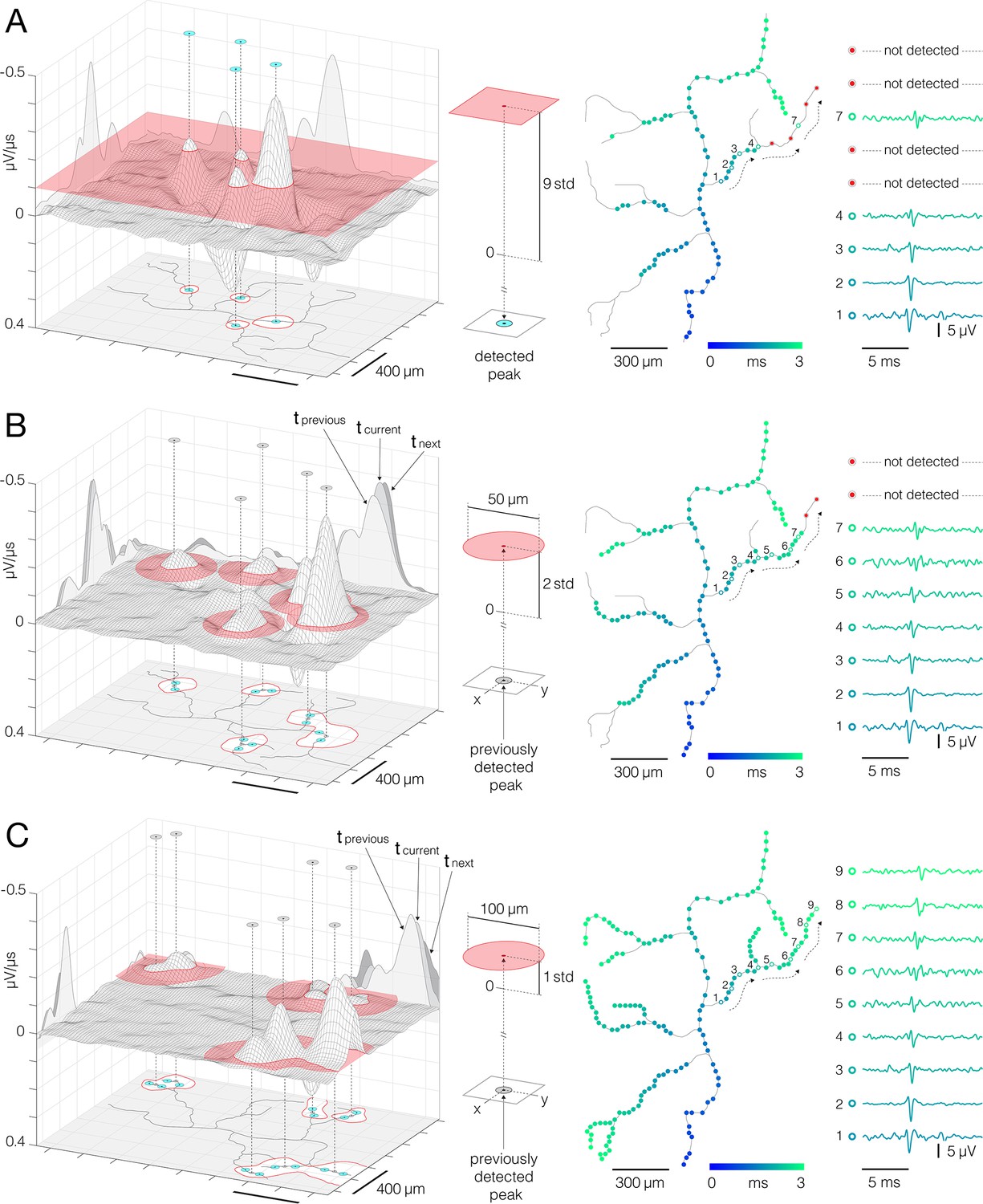
(A) A simple threshold enables detection of high-amplitude signal peaks. (Left) 3D graph shows planar threshold (red semitransparent plane) applied to a section of neuronal signal (3D gray-lined mesh) reconstructed for a single timeframe. 2D profiles of the reconstructed signal are projected on the graph’s side planes (gray-filled hills). Signal cutouts found above the threshold are projected on the graph’s bottom (red-line bordered white patches). Detected signal peaks are denoted by cyan circles projected perpendicularly from top to the bottom of the graph. Axonal contour shown at the graph’s bottom was estimated by observing spatial movements of the signal peaks over consecutive timeframes (also see Figure 6—videos 1 and 2). (Middle) Simple planar threshold was set to 9 STD of the estimated noise; background noise was sampled across all electrodes during periods when the neuron was inactive. (Right) Spatiotemporal distribution of the detected AP peaks (blue-cyan circles) superimposed over axonal contour (same as in the left panel). Timing of the detected peaks is color-coded. AP waveforms recorded at the numbered locations in the upper-right axonal branch are shown on the side. Black-dashed arrows indicate direction of the propagating APs. Red circles denote signal peaks that were not detected by the simple threshold. (B, C) Adaptations of the threshold based on spatial and temporal coordinates of previously detected peaks enabled detection of low-amplitude signals. (Left) Locally applied thresholds (red semitransparent circles) were centered on XY coordinates of previously detected peaks (gray circles projected perpendicularly from top to the bottom of the graph); local thresholds are adapted to detect neighboring peaks at preceding and succeeding timeframes. Neuronal electrical activity reconstructed for a single timeframe (3D gray-lined mesh) is projected on the graph’s side planes (tcurrent); signal profiles of preceding and succeeding timeframes are also projected (tprevious, tnext). Signal cutouts found above the threshold are projected on the graph’s bottom (red-line bordered white patches). Newly detected peaks are denoted by cyan circles projected on the graph’s bottom plane. Axonal contour same as in (A). (Middle) Detection fields of local thresholds are 50 μm (in B) and 100 μm (in C) in radius, and are set to 2 STD (in B) and 1 STD (in C) of the estimated noise. (Right) Same as in (A); note newly mapped peaks detected near proximal axon. Peak detection strategies are comprehensively demonstrated in Figure 3—videos 1–3.
Figure 3—video 1
Mapping signals across axonal arbor – step 1.
Simple planar threshold set to 9 STD of the estimated noise enables detection of high-amplitude action potential (AP) peaks along the axonal arbor. (Left) 3D graph shows planar threshold (red semitransparent plane) applied on a section of neuronal signal (3D gray-lined mesh) reconstructed over consecutive timeframes. 2D profiles of the reconstructed signal are projected on the graph’s side planes (gray-filled hills). Signal cutouts found above the threshold are projected on the graph’s bottom (red-line bordered patches). Detected signal peaks are denoted by green circles projected perpendicularly from top to bottom of the graph. Axonal contour shown at the graph’s bottom was estimated by observing spatial movements of the signal peaks over consecutive timeframes. (Right) 2D representation of the data shown in left. Spatiotemporal distribution of the detected peaks (blue-cyan circles) superimposed over axonal contour (same as in left). Peaks detected over consecutive timeframes are denoted by green circles; detected peaks are embedded within 2D projection of the signal cutouts found above the threshold (red-line bordered patches, same as in left). Occurrence time of detected peaks is color-coded (blue-cyan). Neuronal electrical activity reconstructed over consecutive timeframes is shown in the background; average AP amplitude is color-coded (gray scale). Section of the same data is presented in Figure 3A.
Figure 3—video 2
Mapping signals across axonal arbor – step 2.
Adaptations of the threshold based on spatial and temporal coordinates of previously mapped peaks enable detection of low-amplitude action potentials (APs) along the axonal arbor. (Left) 3D graph shows local thresholds (red semitransparent circles) applied on a section of neuronal signal (3D gray-lined mesh) reconstructed over consecutive timeframes. Local thresholds are centered on XY coordinates of previously detected peaks and are adapted to detect neighboring peaks in preceding and succeeding timeframes; detection fields of local thresholds are 50 μm in radius, and are set to 2 STD of the estimated noise. Signal cutouts found above the threshold are projected on the graph’s bottom (red-line bordered patches). Detected signal peaks are denoted by green circles projected perpendicularly from top to the bottom of the graph. Axonal contour shown at the graph’s bottom was estimated by observing spatial movements of the signal peaks over consecutive timeframes. (Right) 2D representation of the data shown in left. Spatiotemporal distribution of the detected peaks superimposed over axonal contour. Peaks detected over consecutive timeframes are denoted by green circles appearing in each frame; detected peaks are embedded within 2D projection of the signal cutouts found above the threshold (red-line bordered patches, same as in left). Previously detected peaks are denoted by white-filled circles; newly detected peaks are denoted by accumulating blue-cyan circles. Occurrence time of detected peaks is color-coded (blue-cyan). Neuronal electrical activity reconstructed over consecutive timeframes is shown in the background; average AP amplitude is color-coded (gray scale). Section of the same data is presented in Figure 3B.
Figure 3—video 3
Mapping signals across axonal arbor – step 3.
Adaptations of the threshold based on spatial and temporal coordinates of previously mapped peaks enable detection of low-amplitude action potentials (APs) along axonal arbor. (Left) 3D graph shows local thresholds (red semitransparent circles) applied on a section of neuronal signal (3D gray-lined mesh) reconstructed over consecutive timeframes. Local thresholds are centered on XY coordinates of previously detected peaks and are adapted to detect neighboring peaks in preceding and succeeding timeframes; detection fields of local thresholds are 100 μm in radius, and are set to 1 STD of the estimated noise. Signal cutouts found above the threshold are projected on the graph’s bottom (red-line bordered patches). Detected signal peaks are denoted by green circles projected perpendicularly from top to the bottom of the graph. Axonal contour shown at the graph’s bottom was estimated by observing spatial movements of the signal peaks over consecutive timeframes. (Right) 2D representation of the data shown in left. Spatiotemporal distribution of the detected peaks superimposed over axonal contour. Peaks detected over consecutive timeframes are denoted by green circles appearing in each frame; detected peaks are embedded within 2D projection of the signal cutouts found above the threshold (red-line bordered patches, same as in left). Previously detected peaks are denoted by white-filled circles; newly detected peaks are denoted by accumulating blue-cyan circles. Occurrence time of detected peaks is color-coded (blue-cyan). Neuronal electrical activity reconstructed over consecutive timeframes is shown in the background; average AP amplitude is color-coded (gray scale). Section of the same data is presented in Figure 3C.
Figure 4 with 3 supplements

Reconstruction of axonal functional morphology.
(A) Direct interconnection of mapped action potential (AP) peaks. (Left-middle) Closest signal peaks found within a 100 μm Euclidean range (pink-dashed circles) and mapped in two consecutive timeframes (current and preceding peak) were interconnected via direct links (rectilinear white lines). Axonal APs reconstructed for the current timeframe is shown in the background (contour map); average signal amplitude is color-coded (gray scale). (Right) Axonal conduction trajectories revealed by direct interconnection; timing of the propagating AP is color-coded (blue-cyan). (B) Skeletonization-assisted interconnection of mapped signal peaks. (Left-middle) Signal peaks found within a 200 μm Euclidean range (pink-dashed circles) and mapped at two consecutive timeframes (current and preceding peak) are interconnected via remnants of the skeletonized signal (irregular white lines) – signal averaged over the two consecutive timeframes (Δt=100 μs) is skeletonized to infer directionality of the propagating signal. Axonal signal averaged over the two consecutive timeframes is shown in the background (contour map); signal amplitude is color-coded (gray scale). (Right) Axonal conduction trajectories reconstructed using direct and skeletonization-assisted interconnection; timing of the propagating signal is color-coded (blue-cyan). (C) Indirect interconnection of mapped signal peaks. (Left-middle) Signal peaks that were mapped at every other timeframe and found within a 400 μm Euclidean range (pink-dashed circles) were interconnected indirectly – the signal averaged over three consecutive timeframes (Δt=150 μs) was skeletonized to interconnect peaks mapped in first and third timeframe (irregular white line); data for the second timeframe was predicted based on the conduction velocity observed in previously reconstructed trajectories. Axonal signal averaged over the three consecutive timeframes is shown in the background (contour map); signal amplitude is color-coded (gray scale). (Right) Functional axonal morphology reconstructed using direct, skeletonization-assisted and indirect interconnection; timing of the propagating APs is color-coded (blue-cyan). Direct, skeletonization-assisted and indirect interconnections of mapped signal peaks are demonstrated in Figure 4—videos 1–3.
Figure 4—video 1
Direct interconnection of mapped signal peaks.
Fragments of axonal conduction trajectory reconstructed based on spatiotemporal proximities of axonal signal peaks. (Left) Closest signal peaks found within 100 μm Euclidean range (moving white circles) and mapped over consecutive timeframes are interconnected via direct links (transient white lines). Signal peaks found in a current timeframe are denoted by white-filled circles. Signal peaks found in three preceding timeframes are denoted by colored circles (blue-cyan); colors encode signal conduction time. Direct links established in preceding timeframes are presented by thin black lines; direct links outline fragments of axonal conduction trajectory. Non-connected peaks are denoted by black-filled circles. Spontaneous activity of the corresponding neuron is shown in the background; average amplitude of the axonal signal is color-coded (gray scale). (Right) Fragments of axonal conduction trajectory revealed by direct interconnection (as shown in left) are presented by thick colored lines (blue-cyan); colors encode conduction time of axonal signals. Spontaneous activity of the corresponding neuron is shown in the background; average amplitude of the axonal signal is color-coded (gray scale). Section of the same data is presented in Figure 4A.
Figure 4—video 2
Skeletonization-assisted interconnection of mapped signal peaks.
Skeletonized axonal signals mediate interconnection of mapped peaks that could not be interconnected directly. (Left) Fragments of axonal conduction trajectory revealed by direct interconnection (as shown in Figure 4—video 1) are presented through dark-gray contour. Remaining gaps in the trajectory are filled via skeletonization-assisted interconnection of mapped peaks. Signal peaks found within 200 μm Euclidean range (moving white circles) and mapped in two consecutive timeframes are interconnected via remnants of the skeletonized signal (irregular white lines) – signal averaged over the two consecutive timeframes (Δt=100 μs) is skeletonized to infer directionality of the axonal conduction. Signal peaks found in a current timeframe are denoted by white-filled circles. Signal peaks found in the preceding timeframe are denoted by colored circles (blue-cyan); colors encode timing of the signal conduction. Non-connected peaks are denoted by black-filled circles. Spontaneous activity of the corresponding neuron is shown in the background; average amplitude of the axonal signal is color-coded (gray scale). (Right) Axonal conduction trajectory revealed by direct and skeletonization-assisted interconnection (as shown in left) is presented by thick colored lines (blue-cyan); colors encode timing of the signal conduction. Spontaneous activity of the corresponding neuron is shown in the background; average amplitude of the axonal signal is color-coded (gray scale). Section of the same data is presented in Figure 4B.
Figure 4—video 3
Indirect interconnection of mapped signal peaks.
Indirect interconnection enables to interlink spatiotemporally distanced peaks that could not be interconnected via direct nor skeletonization-assisted interconnection. (Left) Axonal conduction trajectory revealed by direct and skeletonization-assisted interconnection (as shown in Figure 4—video 2) are presented through dark-gray contour. Remaining gaps in the trajectory are filled via indirect interconnection of mapped peaks. Spatiotemporally distanced peaks that are mapped in every second timeframe and found within 400 μm Euclidean range (moving white circles) are interconnected indirectly – signal averaged over three consecutive timeframes (Δt=150 μs) is skeletonized to interconnect peaks mapped in first (current) and third (second preceding) timeframe (irregular white lines); data for second (first preceding) timeframe is predicted based on the average conduction velocity observed in previously reconstructed fragments of the trajectory. Signal peaks found in a current timeframe are denoted by white-filled circles. Signal peaks found in the second preceding timeframe are denoted by colored circles (blue-cyan); colors encode timing of the signal conduction. Data predicted for the first preceding timeframe is denoted by framed white-filled circles. Spontaneous activity of the corresponding neuron is shown in the background; average amplitude of the axonal signal is color-coded (gray scale). (Right) Axonal conduction trajectory revealed by direct, skeletonization-assisted and indirect interconnection (as shown in left) is presented by thick colored lines (blue-cyan); colors encode timing of the signal conduction. Spontaneous activity of the corresponding neuron is shown in the background; average amplitude of the axonal signal is color-coded (gray scale). Section of the same data is presented in Figure 4C.
Figure 5
Performances of the algorithm for detection of axonal signal peaks.
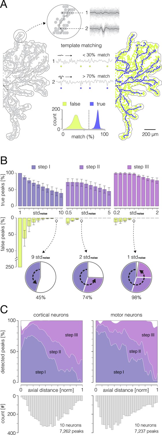
(A) Principle of the template-matching demonstrated on data recorded from cortical axons: (Left) Extracellular action potentials (APs) were spike-sorted (see Figure 2—figure supplement 6) and reconstructed across an entire array (see Figure 2—figure supplement 7) by averaging 100–200 single trials on each electrode. Reconstructed 3D signals were next transformed into derivatives (see Figure 3) and all available signal peaks were obtained. Obtained peaks (pale-gray circles) are superimposed over the contour of axonal morphology. (Middle) Voltage traces recorded at locations of two example peaks are shown at the top (denoted as 1 and 2); averaged templates (black traces) are superimposed over single recording trials (light-gray traces). Note weak similarities in waveforms between the template and single trials at location 1 (putative noise) as oppose to strong similarities at location 2 (putative axonal signal). Template-matching procedure: the waveform of the template is successively compared with waveforms of discrete recording trials to extract percentage of ‘matching’ trials within total number of trials. Examples of recording trials are presented continually within voltage traces (denoted as 1 and 2) and their relative positions are marked by circles: yellow and blue circles denote template mismatches and matches, respectively. Histogram below expresses separability between true and false peaks obtained from the template-matching; all obtained peaks (as shown in left) were used for this analysis. Data that yielded a match of >70% were considered true axonal signal. (Right) True and false peaks (blue and yellow circles, respectively) were classified using the template-matching technique. (B) Performance of the algorithm for AP peak detection. Histograms show percentages of true and false peak detections across the three thresholding steps (see Figure 3) with varying threshold levels. Percentages of true peak detections are exposed through violet, purple, and magenta ascending bars (steps I, II, and III, respectively); percentages of false peak detections are exposed through yellow descending bars. True and false peak detections are expressed as percentages of corresponding peaks detected by the template-matching. Note: no false peak detections were observed at thresholds set to 9, 2, and 1 STD of the noise in steps I, II, and III, respectively. Pie charts below show progress in the true peak detection across the three steps. (C) Detectability of signal peaks across arbors of cortical and motor neuron axons. Detectability for the three steps is expressed over axial distances from the putative axon initial segments (AISes). The bottom histogram shows spatial distribution of detected peaks. Data shown in (B, C) was obtained from 10 cortical and 10 motor neurons.
Figure 6 with 3 supplements

Performances of the algorithm for reconstruction of axonal functional morphology.
(A) Axonal conduction trajectories (black axonal contour) reconstructed from stimulation-triggered neuronal activities; electrical stimulation targeted three different axonal sites (yellow semitransparent circles); red dashed arrows indicate directions of axonal conduction triggered from the corresponding stimulation site. Stimulation-triggered action potentials (APs) were reconstructed across an entire array and presented across consecutive movie frames, enabling visual tracking and reconstruction of axonal conduction trajectories (see Figure 6—videos 1 and 2). (B) Performance of the algorithm for reconstruction of axonal functional morphology. Histograms display percentages of true and false links established between mapped AP peaks using direct, skeletonization-assisted and indirect interconnection (see Figure 3). Percentages of true links are exposed through dark-gray, gray, and pale-gray ascending bars (steps I, II and III, respectively); percentages of false links are exposed through yellow descending bars. Percentages of true and false links obtained using different radii for interconnection of the peaks are shown for each of the steps. The percentages are expressed with respect to a total number of links found in the corresponding ground truth trajectory (as shown in A). Note: no false links were established within Euclidean range (radius) of 100, 200, and 400 μm in steps I, II, and III, respectively. Pie charts below show progress in the reconstruction of axonal morphology across the three steps. (C) Efficiency of the reconstruction (% of connected nodes) estimated for the three interconnection steps. Efficiencies are shown separately for cortical and motor neuron axons and are expressed over axial distances from the putative axon initial segments (AISes). The bottom histogram shows spatial distribution of connected nodes. Data shown in (B, C) was obtained from 10 cortical and 10 motor neurons.
Figure 6—figure supplement 1
Targeted microstimulation of axons using the high-density microelectrode array (HD-MEA) system.
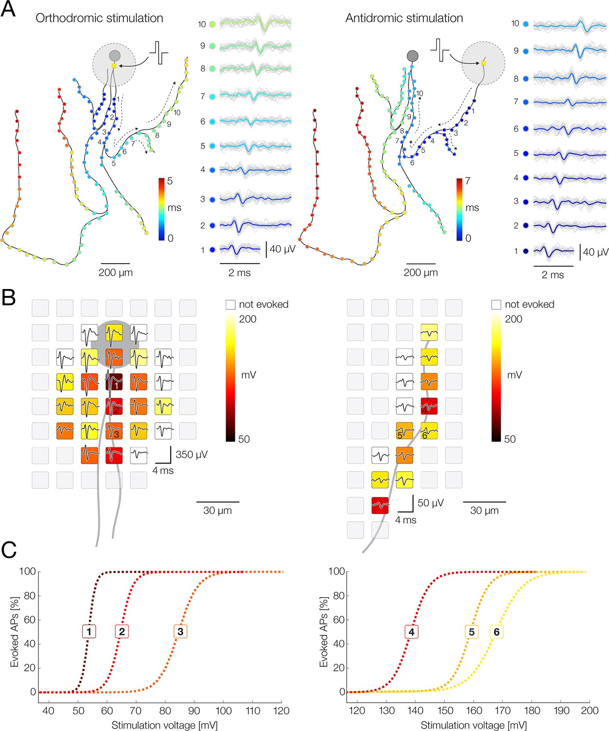
(A) Schematic representation of electrical stimulations directed at proximal (left) and distal (right) axon of a motor neuron. Stimulation-triggered axonal action potentials (APs) are presented through colored circles superimposed over black axonal contour; conduction time of the presented APs is color-coded. Black dashed arrows indicate directions of axonal conduction. Waveforms of axonal APs recorded from 10 denoted locations (1–10) are shown on the sides; averaged waveforms (color-coded traces) are superimposed over single recording trials (pale-gray traces). Positive-first biphasic voltage pulses were used to stimulate the neuron. Stimulation sites are denoted by yellow squares centered within large gray circles; the gray circles represent artifacts induced by the stimulations. (Left) Electrical stimulation targeted at proximal axon initiated an orthodromic signal conduction; stimulation voltage amplitude of ±55 mV was used to stimulate the neuron 60 times at 4 Hz. (Right) Electrical stimulation targeted at distal axon initiated an antidromic signal conduction; stimulation voltage amplitude of ±150 mV was used to stimulate the neuron 60 times at 4 Hz. (B) Identification of stimulation electrodes and voltage magnitudes for orthodromic (left) and antidromic (right) stimulation. Average waveforms of neuronal APs (black traces) recorded from proximal and distal axons are superimposed over corresponding ‘stimulation maps’ – spatial distribution of identified stimulation thresholds for effective activation of the neuron. Stimulation thresholds are color-coded and are assigned to physical location of stimulation electrodes. (Left) Stimulation map obtained near proximal axon. Note: the lowest stimulation threshold colocalized with the neuronal signal with the largest amplitude (putative axon initial segment [AIS]). (Right) Stimulation map obtained near the distal axon. Note larger values of stimulation thresholds as compared with the proximal stimulation map. (Left-right) Stimulation electrodes with the lowest thresholds were used for orthodromic and antidromic stimulations presented in (A). Excitability profiles for six denoted electrodes (1–6) are shown in (C). (C) Excitability profiles of six electrodes with the lowest thresholds for orthodromic (1–3) and antidromic (4–6) stimulation. Each of the electrodes was probed with range of stimulation voltages (±10 to ±300 mV) and stimulation-triggered neuronal response was used to express the excitability profiles. Each of the voltages was applied 100 times per electrode. Stimulation thresholds (color-coded in B) were defined as the minimal voltages that activated the neuron in 100% of the stimulation trials.
Figure 6—video 1
Stimulation-aided reconstruction of axonal conduction trajectories.
Axonal conduction trajectories obtained from stimulation-triggered activities of a single motor neuron. Electrical stimulation was directed at three predefined axonal sites (yellow semitransparent circles) – the axon initial segment (AIS) (stimulation I), distal axon on the right (stimulation II), and distal axon on the left (stimulation III). We used charge-balanced positive-first biphasic voltage pulses with phase durations of 200 μs and amplitudes of ±30, ±50, and ±40 mV for the stimulations I, II, and III, respectively. Each of the axonal sites was stimulated 60 times at 4 Hz. Stimulation sites and amplitudes used specifically for this experiment were previously optimized (see Figure 6—figure supplement 1). Stimulation-triggered activities were reconstructed and averaged across an entire array. Reconstructed activities were mapped spatially across all microelectrodes and temporally over discrete timeframes to produce the movie. Time gap between consecutive timeframes is 50 μs. Average signal amplitude is color-coded (gray scale). Observing the spatial movements of signal peaks in consecutive movie frames enabled us to visually track axonal action potential (AP) conduction in different directions and to reconstruct axonal conduction trajectories. Conduction times of stimulation-triggered APs are color-coded (blue-cyan scale). Conduction trajectories of the same neuron are presented in Figure 6A and in Figure 6—video 2.
Figure 6—video 2
Visually tracked axonal conduction trajectories.
Axonal conduction trajectories obtained from spontaneous and stimulation-triggered activities of a single motor neuron (same neuron as in Figure 6—video 1). Spontaneous neuronal activity was mapped spatially across all microelectrodes and temporally over discrete timeframes to produce the movie shown in the background. Time gap between consecutive timeframes is 50 μs. Average signal amplitude is color-coded (gray scale). Observing the spatial movements of signal peaks in consecutive movie frames enabled us to visually track axonal action potential (AP) conduction and to reconstruct axonal conduction trajectories. Conduction times of tracked APs are color-coded (blue-cyan scale). Conduction trajectories of the same neuron are presented in Figure 6A and in Figure 6—video 1.
Figure 7 with 1 supplement

Functional morphologies of cortical and spinal axons.
(A) Functional morphologies of a cortical (left) and motor neuron axons (right) reconstructed based on spontaneous neuronal activities. Branching orders of reconstructed neurites are color-coded; neuronal somas are presented by black-filled circles. Axon initial segments (AIS) are denoted by thick red lines near somas. Functional morphologies of the two neurons are also presented in Figure 7—video 1. (B) Axonal lengths and active areas. Histograms express density distributions of total axonal lengths, sizes of active areas, and length-to-area quotients. Charts express comparisons between the corresponding values obtained from cortical and motor neurons; horizontal black lines denote mean values, perpendicular black-dashed lines denote standard deviations. (C) Lengths of inter-branching segments and axial distances of branching points. (Up) Histograms express density distributions of lengths of inter-branching segments. (Down) Histograms express density distributions of axial distances of branching points (with respect to corresponding AIS). Charts on the right express comparisons between the corresponding values obtained from cortical and motor neurons; horizontal black lines denote mean values, perpendicular black-dashed lines denote standard deviations. (D) Quantity and axial distances of axon terminals. (Up) Histograms express density distributions of numbers of axon terminals per cell. (Down) Histograms express density distributions of axial distances of axon terminals (with respect to corresponding AIS). Charts on the right express comparisons between the corresponding values obtained from cortical and motor neurons; horizontal black lines denote mean values, perpendicular black-dashed lines denote standard deviations. Color-code: pale-gray color was used to mark data obtained from cortical neurons; dark-gray color was used to mark data obtained from motor neurons. Data shown in (B, C, D) was extracted from functional morphologies of 50 cortical and 50 motor neurons. ***p<0.001.
Figure 7—video 1
Functional morphologies of cortical and spinal axons.
Functional morphologies of cortical (left) and spinal (right) axonal arbors reconstructed based on spontaneous neuronal activities. Branching orders of reconstructed neurites are color-coded (brown scale); neuronal somas are presented by black-filled circles. Spontaneous activities of corresponding neurons are displayed in the background. Amplitudes of electrical signals recorded by individual electrodes are color-coded in gray scale; recorded signals are mapped spatially across all microelectrodes and temporally over discrete timeframes to produce the movie. Propagation time of axonal action potentials (APs) is displayed in upper-left corner. The time gap between consecutive timeframes is 50 μs. Functional morphologies of the two neurons are also presented in Figure 7A.
Figure 8 with 1 supplement

Signal amplitude fluctuations during axonal conduction.
(A) Action potential (AP) waveforms extracted from functional morphologies of cortical and motor neuron axons. (Left) Functional morphology of a single cortical neuron is displayed in gray; average AP amplitudes tracked across selected axonal path are color-coded; waveforms of axonal APs obtained from the denoted locations (numbered 1–13) are shown beside. (Right) Functional morphology of a single motor neuron is displayed in gray; average AP amplitudes tracked across selected axonal path are color-coded; waveforms of axonal APs obtained from the denoted locations (numbered I–XII) are shown beside. Note difference in scalebars for AP waveforms obtained from proximal and distal axons. Data from the two neurons are also presented in Figure 8—video 1. (B) Axonal AP amplitudes versus axial distance from the axon initial segment (AIS). (Left-middle) Amplitudes of axonal APs versus axial distances of their recording sites are plotted for cortical and motor neurons; axial distances are expressed with respect to locations of the corresponding AISes. The black curves represent mean values of amplitudes over all data points. The bottom histograms show density distributions of axial distances from the corresponding AISes. (Right) Mean AP amplitudes obtained from proximal and distal axons are compared between cortical and motor neurons; comparisons are expressed using box plots. The bottom diagrams show criterium for discriminating proximal from distal axonal locations. AP amplitudes averaged over proximal and distal regions of each of the neurons were used in this analysis. (C) Axonal AP amplitudes versus axonal branching order. (Left-middle) Amplitudes of axonal AP versus branching order of corresponding axonal segments are plotted for cortical and motor neurons. The white circles (interconnected by black lines) represent mean values of amplitudes computed for discrete branching orders. The bottom histograms show density distributions of branching orders. (Right) Mean signal amplitudes obtained from primary axonal trunks and axonal trees are compared between cortical and motor neurons; comparisons are expressed using box plots. The bottom diagrams show criterium for discriminating primary axonal trunks from axonal trees. Color-code: pale-gray color was used to mark data obtained from cortical neurons; dark-gray color was used to mark data obtained from motor neurons. Data shown in (B, C) was extracted from functional morphologies of 50 cortical and 50 motor neurons. **p<0.01; ***p<0.001.
Figure 8—video 1
Action potential (AP) waveforms as traced across axonal functional morphologies.
Examples of AP waveforms extracted from functional morphologies of cortical (left) and motor neuron (right) axons. (Left) Functional morphology of a cortical axon (white axonal contour) is displayed over spontaneous activity of the corresponding neuron; neuronal soma is presented by black-filled circle. AP waveforms traced across selected axonal path are displayed beside; average AP amplitudes are color-coded. (Right) Functional morphology of a motor neuron axon (white axonal contour) is displayed over spontaneous activity of the corresponding neuron; neuronal soma is presented by black-filled circle. AP waveforms traced across selected axonal path are displayed beside; average AP amplitudes are color-coded. (Middle) Note difference in scalebars for AP waveforms obtained from proximal and distal axons. Functional morphologies of the two neurons are also presented in Figure 8A.
Figure 9
Temporal dynamics of axonal conduction.
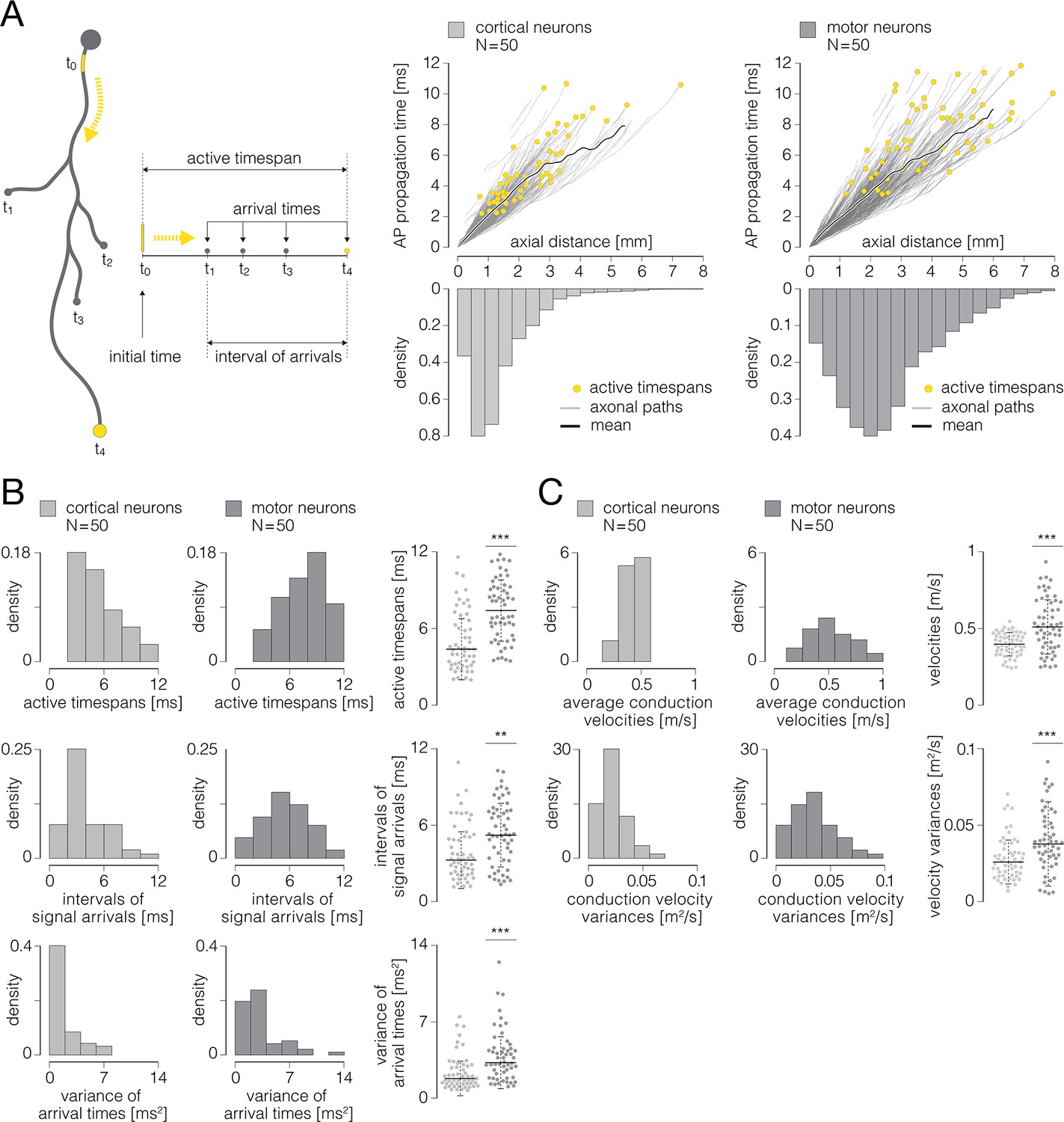
(A) (Left) Graphical representation of parameters that were used for the analysis of temporal aspects of axonal conduction. Thick gray contour represents simplified axonal morphology; neuronal somas are presented by gray-filled circles; a yellow line superimposed over a proximal axon represents the axon initial segment (AIS); blebs at the ends of four axonal branches represent axon terminals. Yellow-dashed arrows indicate directionality of axonal action potential (AP) propagation. Temporal parameters: initial time (t0) – time of the initiation of axonal conduction; arrival times (t1-4) – times at which axonal APs arrive at axon terminals; interval of arrivals – interval between the earliest and the latest arrival time; active timespan – timespan between initial time and the latest arrival time. (Right) Axonal AP propagation time versus axial distance from the AIS – comparison between cortical (graph on the left) and motor neurons (graph on the right). Yellow circles represent active timespans; gray curves in the background represent AP propagation times observed over individual axonal paths; thick black curves represent mean values of propagation times averaged over all axonal paths. (B) Temporal aspects of axonal conduction. (Up) Histograms express density distributions of active timespans for cortical and motor neurons. (Middle) Histograms express density distributions of intervals of arrivals for cortical and motor neurons. (Down) Histograms express density distributions of variances of arrival times for cortical and motor neurons. Charts on the right express comparisons between the corresponding values obtained from cortical and motor neurons; horizontal black lines denote mean values, perpendicular black-dashed lines denote standard deviations. (C) Axonal conduction velocities. (Up) Histograms express density distributions of average conduction velocities for cortical and motor neurons; average velocities are computed for individual cells. (Down) Histograms express density distributions of variances of conduction velocities for cortical and motor neurons; variances are computed for individual cells. Charts on the right express comparisons between the corresponding values obtained from cortical and motor neurons; horizontal black lines denote mean values, perpendicular black-dashed lines denote standard deviations. Color-code: pale-gray color was used to mark data obtained from cortical neurons; dark-gray color was used to mark data obtained from motor neurons. Data shown was extracted from functional morphologies of 50 cortical and 50 motor neurons. **p<0.01; ***p<0.001.
Tables
Key resources table
| Reagent type (species) or resource | Designation | Source or reference | Identifiers | Additional information |
|---|---|---|---|---|
| Strain, strain background (Rattus norvegicus) | Sprague Dawley rat | Charles River Laboratories | Strain Code: 400 | – |
| Cell line (Rattus norvegicus) | Cortical; Spinal | This paper | – | Primary |
| Antibody | Anti-Map2 (Chicken Polyclonal) | Abcam | ab5392 | IHC (1:1000) |
| Antibody | Anti-β-III tubulin (Rabbit Polyclonal) | Abcam | ab18207 | IHC (1:500) |
| Antibody | Anti-mCherry (Mouse Monoclonal) | Abcam | ab125096 | IHC (1:500) |
| Antibody | Alexa Fluor 488 (Goat Anti-Chicken Polyclonal) | Abcam | ab150173 | IHC (1:200) |
| Antibody | Alexa Fluor 488 (Donkey Anti-Rabbit Polyclonal) | Abcam | ab150073 | IHC (1:200) |
| Antibody | Alexa Fluor 594 (Goat Anti-Mouse Polyclonal) | Abcam | ab150116 | 1 IHC (:200) |
| Recombinant DNA reagent | pAAV-hSyn-mCherry | Addgene | Plasmid # 114472 | – |
| Peptide, recombinant protein | Human recombinant laminin | BioLamina | LN211 | – |
| Software, algorithm | Spyking Circus | Yger et al., 2018 | Spyking Circus | Version 1.0.1 |
Additional files
Download links
A two-part list of links to download the article, or parts of the article, in various formats.
Downloads (link to download the article as PDF)
Open citations (links to open the citations from this article in various online reference manager services)
Cite this article (links to download the citations from this article in formats compatible with various reference manager tools)
Functional imaging of conduction dynamics in cortical and spinal axons
eLife 12:e86512.
https://doi.org/10.7554/eLife.86512


